
7.7. Truth-matching#
7.7.1. MC matching#
Important
If you use MC matching for your analysis, please cite the following proceeding Monte Carlo matching in the Belle II software which describes the Belle II MC matching algorithm.
First, you must run it#
MCMatching relates Particle and MCParticle objects.
Important
Most MC matching variables will have non-trivial values only if the MCMatcherParticles module is actually executed.
It can be executed by adding the module to your path, there is a modularAnalysis.matchMCTruth convenience function to do this.
Core#
MC matching at Belle II returns two important pieces of information:
the true PDG id of the particle mcPDG,
and an error flag mcErrors.
Both variables will have non-trivial values only if the MCMatching module,
which relates composite Particle (s) and MCParticle (s), is executed.
mcPDG is set to the PDG code of the first common mother MCParticle of the daughters of this Particle.
- mcErrors[source]
Returns the bit pattern indicating the quality of MC matching.
Note
The bit pattern is explained in Error flags.
- Group:
MC matching and MC truth
- mcPDG[source]
Returns the PDG code of matched MC particle or
NaNif no match could be found.Attention
This requires running
matchMCTruth()either on the reconstructed particle, or one of its ancestors, or a particle list filled with MC particle objects.- Group:
MC matching and MC truth
Extra variables#
There are several extra variables relating to MCMatching.
Many are defined for convenience and can be recreated logically from mcPDG and mcErrors.
Some extra variables are provided externally, for example isCloneTrack from the tracking-level MC matching.
- genNMissingDaughter(PDG)[source]
Returns the number of missing daughters with the specified PDG code, or
NaNif no related MC particle could be found.- Group:
MC matching and MC truth
- genNStepsToDaughter(i)[source]
Returns the number of steps to \(i\)-th daughter of the particle at generator level, or
NaNif no MC particle is associated to the particle or \(i\)-th daughter, or if the \(i\)-th daughter does not exist.- Group:
MC matching and MC truth
- isCloneTrack[source]
Returns 1 if the charged final state particle comes from a cloned track, 0 if it does not come from a clone, and
NaNif the particle is neutral, composite, or no MC particle could be found.- Group:
MC matching and MC truth
- isMisidentified[source]
Returns 1 if the particle is mis-identified (the wrong PDG code is assigned), 0 if PDG code is correct, and
NaNif no related MC particle could be found.- Group:
MC matching and MC truth
- isOrHasCloneTrack[source]
Returns 1 if the particle is a clone track or has a clone track as a daughter, 0 otherwise.
- Group:
MC matching and MC truth
- isSignal[source]
Returns 1.0 if the particle is correctly reconstructed, 0.0 if not, and
NaNif no related MC particle could be found.- Group:
MC matching and MC truth
- isSignalAcceptMissing[source]
Returns 1.0 if the particle is almost correctly reconstructed (missing particles are allowed), 0.0 if not, and
NaNif no related MC particle could be found.- Group:
MC matching and MC truth
- isSignalAcceptMissingGamma[source]
Returns 1.0 if the particle is almost correctly reconstructed (missing photons are allowed), 0.0 if not, and
NaNif no related MC particle could be found.- Group:
MC matching and MC truth
- isSignalAcceptMissingMassive[source]
Returns 1.0 if the particle is almost correctly reconstructed (missing massive particles are allowed), 0.0 if not, and
NaNif no related MC particle could be found.- Group:
MC matching and MC truth
- isSignalAcceptMissingNeutrino[source]
Returns 1.0 if the particle is almost correctly reconstructed (missing neutrinos are allowed), 0.0 if not, and
NaNif no related MC particle could be found.- Group:
MC matching and MC truth
- isSignalAcceptWrongFSPs[source]
Returns 1.0 if the particle is almost correctly reconstructed (mis-identified final state particles are allowed), 0.0 if not, and
NaNif no related MC particle could be found.- Group:
MC matching and MC truth
- isWrongCharge[source]
Returns 1 if the charge of the particle is wrongly assigned, 0 if it’s the correct charge, and
NaNif no related MC particle could be found.- Group:
MC matching and MC truth
Particle Status Flag#
The status flag mcParticleStatus is a bit set where each bit flag
describes a specific property or simulation state of the corresponding MCParticle.
The individual flags are defined by the MCParticle::StatusBit enum.
A value of mcParticleStatus equal to 0 means that none of the predefined
status conditions are set for the particle.
These flags can be used to identify special categories of particles, such as primary particles generated by the event generator, particles that left or stopped inside the detector volume, virtual particles that are not propagated to Geant4, or photons originating from ISR, FSR, or PHOTOS radiation processes. Since the status is encoded as a bit mask, multiple flags can be set simultaneously for a single particle.
Flag |
Explanation |
|---|---|
c_PrimaryParticle = 1 |
Particle is a primary particle produced by the event generator. |
c_StableInGenerator = 2 |
Particle is stable in the generator, i.e. it does not decay during event generation. |
c_LeftDetector = 4 |
Particle left the detector simulation volume. |
c_StoppedInDetector = 8 |
Particle was stopped inside the detector simulation volume. |
c_IsVirtual = 16 |
Particle is virtual and is not propagated to Geant4 (e.g. exchange bosons or off-shell states). |
c_Initial = 32 |
Particle is an initial-state particle such as the incoming \(e^+\) or \(e^-\). |
c_IsISRPhoton = 64 |
Particle is a photon produced by initial state radiation (ISR). |
c_IsFSRPhoton = 128 |
Particle is a photon produced by final state radiation (FSR). |
c_IsPHOTOSPhoton = 256 |
Particle is a radiative photon produced by PHOTOS. |
c_IsRadiativePhoton = 448 |
Combined flag identifying ISR, FSR, or PHOTOS photons. |
Error flags#
The error flag mcErrors is a bit set where each bit flag describes
a different kind of discrepancy between reconstruction and MCParticle.
The individual flags are described by the MCMatching::MCErrorFlags enum.
A value of mcErrors equal to 0 indicates perfect reconstruction (signal).
Usually candidates with only FSR photons missing are also considered as signal,
so you might want to ignore the corresponding c_MissFSR flag.
The same is true for c_MissingResonance, which is set for any missing composite particle (e.g. \(K_1\), but also \(D^{*0}\)).
The behavior of mcErrors can be configured by decay string grammar with modularAnalysis.reconstructDecay().
For more information and examples how to use the decay strings correctly, please see DecayString and Grammar for custom MCMatching.
Full documentation of the MCMatching algorithm is described in BELLE2-CONF-PROC-2022-004.
Flag |
Explanation |
|---|---|
c_Correct = 0 |
This Particle and all its daughters are perfectly reconstructed. |
c_MissFSR = 1 |
A Final State Radiation (FSR) photon is not reconstructed (based on MCParticle: :c_IsFSRPhoton). |
c_MissingResonance = 2 |
The associated MCParticle decay contained additional non-final-state particles (e.g. a rho) that weren’t reconstructed. This is probably O.K. in most cases. |
c_DecayInFlight = 4 |
A Particle was reconstructed from the secondary decay product of the actual particle. This means that a wrong hypothesis was used to reconstruct it, which e.g. for tracks might mean a pion hypothesis was used for a secondary electron. |
c_MissNeutrino = 8 |
A neutrino is missing (not reconstructed). |
c_MissGamma = 16 |
A photon (not FSR) is missing (not reconstructed). |
c_MissMassiveParticle = 32 |
A generated massive FSP is missing (not reconstructed). |
c_MissKlong = 64 |
A Klong is missing (not reconstructed). |
c_MisID = 128 |
One of the charged final state particles is mis-identified (wrong signed PDG code). |
c_AddedWrongParticle = 256 |
A non-FSP Particle has wrong PDG code, meaning one of the daughters (or their daughters) belongs to another Particle. |
c_InternalError = 512 |
No valid match was found. For tracks, it indicates that there is not a true track related to the reconstructed one. Might indicate fake or background track or cluster. |
c_MissPHOTOS = 1024 |
A photon created by PHOTOS was not reconstructed (based on MCParticle: :c_IsPHOTOSPhoton). |
c_AddedRecoBremsPhoton = 2048 |
A photon added with the bremsstrahlung recovery tools (correctBrems or correctBremsBelle) has no MC particle assigned, or it doesn’t belong to the decay chain of the corrected lepton mother |
Example of use#
The two variables together allow the user not only to distinguish signal (correctly reconstructed)
and background (incorrectly reconstructed) candidates, but also to study and identify various types of physics background
(e.g. mis-ID, partly reconstructed decays, …).
To select candidates that have a certain flag set, you can use bitwise and to select only this flag from mcErrors
and check if this value is non-zero: (mcErrors & MCMatching::c_MisID) != 0 .
For use in a TTree selector, you’ll need to use the integer value of the flag instead:
ntuple->Draw("M", "(mcErrors & 128) != 0")
You can also make use of MCMatching::explainFlags() which prints a human-readable
list of flags present in a given bitset. Can also be used in both C++ and python:
If instead only binary decision (1 = signal, 0 = background) is needed,
then for convenience one can use isSignal (or isSignalAcceptMissingNeutrino for semileptonic decays).
from modularAnalysis import variablesToNtuple
variablesToNtuple("X:mycandidates -> Y Z", variables = ["isSignal"] + other_interesting_variables)
assuming you have reconstructed X -> Y Z :
from modularAnalysis import applyCuts
applyCuts('X:myCandidates', 'isSignal==1')
7.7.2. MC decay finder module ParticleCombinerFromMC#
Analysis module to reconstruct a given decay using the list of generated particles MCParticle. Only signal particles with isSignal equal to 1 are stored.
The module can be used for:
Determination of the number of generated decays for efficiency studies, especially in the case of inclusive decays (e.g.: What’s the generated number of \(B \to D^0 X\) decays?).
Matched MC decays as input for a truth matching module.
import basf2

# Create main path
main = basf2.create_path()

# Modules to generate events, etc.
...

import modularAnalysis as ma

# Load particles from MCParticle at first
ma.fillParticleListFromMC('K+:MC',    '', path=main)
ma.fillParticleListFromMC('pi+:MC',   '', path=main)
ma.fillParticleListFromMC('e+:MC',    '', path=main)
ma.fillParticleListFromMC('nu_e:MC',  '', path=main)
ma.fillParticleListFromMC('gamma:MC', '', path=main)

"""
Example 1
Search for B+ decaying to anti-D0* e+ nu_e, where anti-D0* decays to [anti-D0 -> K+ pi- pi0] and pi0.
Additional photons emitted are ignored. Charge conjugated decays are matched, too.
"""
# Reconstruct pi0 from gamma gamma at fist for convenience. Then reconstruct B+ with pi0:gg.
ma.reconstructMCDecay('pi0:gg =direct=> gamma:MC gamma:MC', '', path=main)
ma.reconstructMCDecay(
  'B+:DstENu =direct=> [anti-D*0:D0pi0 =direct=> [anti-D0:Kpipi0 =direct=> K+:MC pi-:MC pi0:gg] pi0:gg ] e+:MC nu_e:MC ',
  '',
  path=main)

# One can directly reconstruct pi0:gg in same decay string.
# But in this case, one have to write sub-decay of pi0:gg only once. Otherwise same particles are registered twice.
# ma.reconstructMCDecay(
#     'B+:DstENu =direct=>\
#      [anti-D*0:D0pi0 =direct=> [anti-D0:Kpipi0 =direct=> K+:MC pi-:MC [pi0:gg =direct=> gamma:MC gamma:MC]] pi0:gg ]\
#      e+:MC nu_e:MC ',
#     '',
#     path=main)


"""
Example 2
Search for B+ decaying to anti-D0 + anything, where the anti-D0 decays to K+ pi-.
Ignore additional photons emitted in the anti-D0 decay. Charge conjugated decays
are matched, too. If there is a match found, save to ParticleList 'B+:testB'
"""
# Reconstruct B+ from [anti-D0 =direct=> K+ pi-] accepting missing daughters
ma.reconstructMCDecay('B+:D0Kpi =direct=> [anti-D0:Kpi =direct=> K+:MC pi-:MC] ... ?gamma ?nu', '', path=main)


...
For more information and examples how to use the decay strings correctly, please see DecayString and Grammar for custom MCMatching.
7.7.3. MC decay finder module MCDecayFinder#
Analysis module to search for a given decay in the list of generated particles MCParticle.
The module can be used for:
Determination of the number of generated decays for efficiency studies, especially in the case of inclusive decays (e.g.: What’s the generated number of \(B \to D^0 X\) decays?).
Matched MC decays as input for a truth matching module.
import basf2

# Create main path
main = basf2.create_path()

# Modules to generate events, etc.
...

import modularAnalysis as ma
# Search for B+ decaying to anti-D0 + anything, where the anti-D0 decays to K+ pi-.
# Ignore additional photons emitted in the anti-D0 decay. Charge conjugated decays
# are matched, too. If there is a match found, save to ParticleList 'B+:testB'
ma.findMCDecay('B+:testB', 'B+ =direct=> [anti-D0 =direct=> K+ pi-] ... ?gamma ?nu', path=main)

# Modules which can use the matched decays saved as Particle in the ParticleList 'B+:testB'
...
For more information and examples how to use the decay strings correctly, please see DecayString and Grammar for custom MCMatching.
Compact decay strings per event#
The PrintMCParticles module (used via modularAnalysis.printMCParticles) can store a compact,
single-line representation of the generated decay tree of each event in the __MCDecayString__ branch,
by setting storeCompact=True instead of using the default indented multi-line tree:
import modularAnalysis as ma
ma.printMCParticles(storeCompact=True, onlyPrimaries=True, suppressPrint=True, path=main)
A typical value of the resulting string for a generic \(\Upsilon(4S) \to B\bar{B}\) event looks like:
Upsilon(4S) -> [B+ -> mu+ nu_mu gamma] [B- -> pi- [D0 -> pi- pi+]]
For non-\(\Upsilon(4S)\) events, e.g. continuum \(e^+e^- \to c\bar{c}\) events, the top-level particles are instead the initial-state beam particles and the intermediate boson they produce, since these also have no mother particle in the generated event, for example:
e- e+ Z0 -> [D*+ -> [D0 -> [K_S0 -> pi+ pi-] pi+ pi- pi+ pi-] pi+] [pi0 -> gamma gamma] [rho- -> pi- [pi0 -> gamma gamma]] pi+ [D- -> K_L0 pi-]
Here -> separates a particle from its daughters, [...] groups a composite daughter together with
its own descendants, and ~ prefixes secondary particles (i.e. particles created during the detector
simulation rather than by the generator). A particle whose PDG code is not known to TDatabasePDG is
named UNKNOWN(<pdg code>).
Radiative photons are also given a distinct name so that they can be told apart from generator-level photons when parsing the string:
gammaIfor initial state radiation (based on MCParticle:c_IsISRPhoton),gammaFfor final state radiation (based on MCParticle:c_IsFSRPhoton),gammaPfor photons added by PHOTOS (based on MCParticle:c_IsPHOTOSPhoton),
For example, if the muon in the decay above also radiated a PHOTOS photon:
Upsilon(4S) -> [B+ -> mu+ nu_mu gamma gammaP] [B- -> pi- [D0 -> pi- pi+]]
By default onlyPrimaries is False, so secondary particles are also included in the string, for
example if the primary \(\pi^-\) above instead interacted in the detector material:
Upsilon(4S) -> [B+ -> mu+ nu_mu gamma] [B- -> [pi- -> ~gamma ~gamma] [D0 -> pi- pi+]]
Setting onlyPrimaries=True (as in the first example) omits such secondary particles and their
descendants entirely, which is usually the more useful setting for studying the generated decay itself.
If maxLevel limits the depth of the tree, a particle whose daughters are cut off by this limit has
-> ... appended after it instead of showing its daughters, mirroring the → … indicator used in
the default indented tree. For example, applying maxLevel=1 to the first example above would collapse
it to:
Upsilon(4S) -> ...
This truncation does not happen by default, since the default maxLevel=-1 means the tree is never cut
off.
Because this string is written out per event, it can be stored
alongside the other analysis variables (e.g. via modularAnalysis.variablesToNtuple) and then parsed
offline, for example with a simple recursive-descent parser or even just string/regular-expression
matching on the particle names, to study which decay chains actually occurred in each generated event.
Unlike the numbered generated decay modes described below, this does not require every mode of interest
to be enumerated in advance.
Important
When running on all events, it is important to also set suppressPrint=True (as in the
example above). Otherwise the default indented tree is still built and printed via B2INFO
for every event, in addition to being stored in storeCompact format, which can cause the
log files to explode in size.
7.7.4. Generated decay modes#
A tool has been developed which analyzes the array of MC particles and determines the generated decay mode of the event.
Compared to storing the full decay string (as described above), storing this decay mode number is a much more efficient way to record the generated decay of an event, since only a single integer needs to be saved instead of a string. However, this efficiency comes at the cost of flexibility: only the decay modes enumerated below are recognized, and this hardcoded mapping is limited to the decay modes explicitly generated by EvtGen for B decays. It does not cover decay modes generated by Pythia.
A total of 825 \(B^+\) decay modes have been defined:
The first 80 numbers are semi-leptonic decays (\(B^+ \to h l^+ \nu_l\)), e.g.
1001: \(B^+ \to \bar{D^{*0}} e^+ \nu_e\)
1002: \(B^+ \to \bar{D^0} e^+ \nu_e\)
1003: \(B^+ \to \bar{D_1^0} e^+ \nu_e\)
The numbers 1085 to 1092 are radiative decays.
There are 17 \(B^+ \to X l^+ l^-\) decay modes.
The numbers 1113 to 1608 are hadronic charmless decays.
Then there are 70 charmonium decays with \(J/\psi\), \(\Psi(2S)\), \(\eta_c\), etc.
This is followed by decays involving two or one charm meson.
The last 17 decay modes involve baryons.
The same number of \(B^-\) decay modes have been implemented. They have negative tags.
- BminusMode[source]#
[Eventbased] Returns the decay modes of \(B^-\) particles.
Note
The list of decay modes is documented in Generated decay modes.
- Group:
MCParticle tag variables
- BplusMode[source]#
[Eventbased] Returns the decay modes of \(B^+\) particles.
Note
The list of decay modes is documented in Generated decay modes.
- Group:
MCParticle tag variables
The same general structure is used for the 1000 \(B^0\) and \(\bar{B^0}\) modes accessible via the variables
- B0Mode[source]#
[Eventbased] Returns the decay modes of \(B^0\) particles.
Note
The list of decay modes is documented in Generated decay modes.
- Group:
MCParticle tag variables
- Bbar0Mode[source]#
[Eventbased] Returns the decay modes of \(\overline{B}{}^0\) particles”.
Note
The list of decay modes is documented in Generated decay modes.
- Group:
MCParticle tag variables
For \(B_s^0\) and \(\bar{B_s^0}\) a total of 264 decay have been defined.
- Bs0Mode[source]#
[Eventbased] Returns the decays mode of \(B^0_s\) particles.
Note
The list of decay modes is documented in Generated decay modes.
- Group:
MCParticle tag variables
- Bsbar0Mode[source]#
[Eventbased] Returns the decay modes of \(\overline{B}{}^0_s\) particles.
Note
The list of decay modes is documented in Generated decay modes.
- Group:
MCParticle tag variables
Besides the B meson decays three \(D^{*\pm}\), 84 \(D_s^\pm\), 84 \(D^\pm\), and 136 \(D^0\) charm meson decays are implemented. For each category the tag number starts again at 1001.
- D0Mode[source]#
[Eventbased] Returns the decay modes of \(D^0\) particles.
Note
The list of decay modes is documented in Generated decay modes.
- Group:
MCParticle tag variables
- Dbar0Mode[source]#
[Eventbased] Returns the decay modes of \(\overline{D}{}^0\) particles.
Note
The list of decay modes is documented in Generated decay modes.
- Group:
MCParticle tag variables
- DminusMode[source]#
[Eventbased] Returns the decay modes of \(D^-\) particles.
Note
The list of decay modes is documented in Generated decay modes.
- Group:
MCParticle tag variables
- DplusMode[source]#
[Eventbased] Returns the decay modes of \(D^+\) particles.
Note
The list of decay modes is documented in Generated decay modes.
- Group:
MCParticle tag variables
- DsminusMode[source]#
[Eventbased] Returns the decay modes of \(D^-_s\) particles.
Note
The list of decay modes is documented in Generated decay modes.
- Group:
MCParticle tag variables
- DsplusMode[source]#
[Eventbased] Returns the decay modes of \(D^+_s\) particles.
Note
The list of decay modes is documented in Generated decay modes.
- Group:
MCParticle tag variables
- DstminusMode[source]#
[Eventbased] Returns the decay modes of \(D^{*-}\) particles.
Note
The list of decay modes is documented in Generated decay modes.
- Group:
MCParticle tag variables
- DstplusMode[source]#
[Eventbased] Returns the decay modes of \(D^{*+}\) particles.
Note
The list of decay modes is documented in Generated decay modes.
- Group:
MCParticle tag variables
The full list of all decay modes can be found in the technical Belle note BELLE2-NOTE-TE-2021-002.
7.7.5. Tau decay MC modes#
A special case is the decay of generated tau lepton pairs. For their study, it is useful to call the function labelTauPairMC in the steering file.
from modularAnalysis import labelTauPairMC
labelTauPairMC()
- tauMinusMCMode[source]#
[Eventbased] Returns the decay ID for the negative \(\tau\) lepton in a \(\tau\tau\) generated event.
Attention
Calculating this variable requires using the
TauDecayMarkerModulein your steering file.Note
The list of decay modes is documented in Tau decay MC modes.
- Group:
Generated tau decay information
- tauMinusMCProng[source]#
[Eventbased] Returns the prong for the negative \(\tau\) lepton in a \(\tau\tau\) generated event.
Attention
Calculating this variable requires using the
TauDecayMarkerModulein your steering file.Note
The list of decay modes is documented in Tau decay MC modes.
- Group:
Generated tau decay information
- tauPlusMCMode[source]#
[Eventbased] Returns the decay ID for the positive \(\tau\) lepton in a \(\tau\tau\) generated event.”
Attention
Calculating this variable requires using the
TauDecayMarkerModulein your steering file.Note
The list of decay modes is documented in Tau decay MC modes.
- Group:
Generated tau decay information
- tauPlusMCProng[source]#
[Eventbased] Returns the prong for the positive \(\tau\) lepton in a \(\tau\tau\) generated event.
Attention
Calculating this variable requires using the
TauDecayMarkerModulein your steering file.Note
The list of decay modes is documented in Tau decay MC modes.
- Group:
Generated tau decay information
Using MC information, labelTauPairMC identifies if the generated event is a tau pair decay.
The variables tauPlusMCProng and tauMinusMCProng store the prong (number of final state charged particles) coming from each one of the generated tau leptons. If the event is not a tau pair decay, the value in each one of these variables will be 0.
The channel number will be stored in the variables tauPlusMCMode, and tauMinusMCMode (one for the positive and the other for the negative) according to the following tables.
TauolaBelle2 Decay Modes#
The table for TauolaBelle2 can be found in the note BELLE2-NOTE-PH-2020-055.
TauolaBelle Decay Modes#
MC mode |
Decay channel |
MC mode |
Decay channel |
|---|---|---|---|
-1 |
Not a tau pair event |
24 |
\(\tau^- \to \pi^- \omega \pi^0 \nu\) |
1 |
\(\tau^- \to e^- \nu \bar{\nu}\) |
25 |
\(\tau^- \to \pi^- \pi^+ \pi^- \eta \nu\) |
2 |
\(\tau^- \to \mu^- \nu \bar{\nu}\) |
26 |
\(\tau^- \to \pi^- \pi^0 \pi^0 \eta \nu\) |
3 |
\(\tau^- \to \pi^- \nu\) |
27 |
\(\tau^- \to K^- \eta \nu\) |
4 |
\(\tau^- \to \rho^- \nu\) |
28 |
\(\tau^- \to K^{*-} \eta \nu\) |
5 |
\(\tau^- \to a_1^- \nu\) |
29 |
\(\tau^- \to K^- \pi^+ \pi^- \pi^0 \nu\) |
6 |
\(\tau^- \to K^- \nu\) |
30 |
\(\tau^- \to K^- \pi^0 \pi^0 \pi^0 \nu\) |
7 |
\(\tau^- \to K^{*-} \nu\) |
31 |
\(\tau^- \to K^0 \pi^- \pi^+ \pi^- \nu\) |
8 |
\(\tau^- \to \pi^- \pi^+ \pi^- \pi^0 \nu\) |
32 |
\(\tau^- \to \pi^- \bar{K}^0 \pi^0 \pi^0 \nu\) |
9 |
\(\tau^- \to \pi^- \pi^0 \pi^0 \pi^0 \nu\) |
33 |
\(\tau^- \to \pi^- K^+ K^- \pi^0 \nu\) |
10 |
\(\tau^- \to 2\pi^- \pi^+ 2\pi^0 \nu\) |
34 |
\(\tau^- \to \pi^- K^0 \bar{K}^0 \pi^0 \nu\) |
11 |
\(\tau^- \to 3\pi^- 2\pi^+ \nu\) |
35 |
\(\tau^- \to \pi^- \omega \pi^+ \pi^- \nu\) |
12 |
\(\tau^- \to 3\pi^- 2\pi^+ \pi^0 \nu\) |
36 |
\(\tau^- \to \pi^- \omega \pi^0 \pi^0 \nu\) |
13 |
\(\tau^- \to 2\pi^- \pi^+ 3\pi^0 \nu\) |
37 |
\(\tau^- \to e^- e^- e^+ \nu \bar{\nu}\) |
14 |
\(\tau^- \to K^- \pi^- K^+ \nu\) |
38 |
\(\tau^- \to f_1 \pi^- \nu\) |
15 |
\(\tau^- \to K^0 \pi^- K^0bar \nu\) |
39 |
\(\tau^- \to K^- \omega \nu\) |
16 |
\(\tau^- \to K^- K^0 \pi^0 \nu\) |
40 |
\(\tau^- \to K^- K^0 \pi^+ \pi^- \nu\) |
17 |
\(\tau^- \to K^- \pi^0 \pi^0 \nu\) |
41 |
\(\tau^- \to K^- K^0 \pi^0 \pi^0 \nu\) |
18 |
\(\tau^- \to K^- \pi^- \pi^+ \nu\) |
42 |
\(\tau^- \to \pi^- K^+ \bar{K}^0 \pi^- \nu\) |
19 |
\(\tau^- \to \pi^- \bar{K}^0 \pi^0 \nu\) |
||
20 |
\(\tau^- \to \eta \pi^- \pi^0 \nu\) |
||
21 |
\(\tau^- \to \pi^- \pi^0 \gamma \nu\) |
||
22 |
\(\tau^- \to K^- K^0 \nu\) |
||
23 |
\(\tau^- \to \pi^- 4\pi^0 \nu\) |
7.7.6. Track matching#
A reconstructed track can be:
matched, the reconstructed track is matched to a true track, and it is its best description.
clone, the reconstructed track is matched to a true track, but there is another reconstructed track that better describes the true track (this second reconstructed track will therefore be matched)
fake, the reconstructed track is not matched to any true track. It can be a beam-background track or a track built out of noise hits in the detector, or a mixture of these two.
Note
In case of matched or clone tracks, the charge of the reconstructed track is not checked against the charge of the true track. The charge check is anyway included in the MCMatching that sets the Error flags.
More details on the track matching can be found in the trk_matching section of the Tracking chapter, in particular trk_matching_analysis. Here is a table to translate the matching status at tracking level with the one at analysis level:
tracking-level |
analysis-level |
|---|---|
matched |
matched |
wrongCharge |
matched |
clone |
clone |
cloneWrongCharge |
clone |
background |
fake |
ghost |
fake |
7.7.7. MCMatching of ECL clusters#
To understand the method of ECL cluster matching, a basic introduction to the ECL objects used during the reconstruction of simulated data is required.
From the ECLSimHits taken from the GEANT4 simulation, ECLDigits are created and then calibrated to make ECLCalDigit objects which store the energy and
time of a single ECL crystal. The ECLCalDigits are then grouped to make ECLShower objects.
This grouping is represented with weighted relations between an ECLShower and a subset of ECLCalDigits.
The energies of the shower objects are corrected such that, for simulated photons, the peak of the reconstructed energy distribution coincides with the generated photon energy.
The shower objects are also used to calculate shower-shape quantities and certain particle likelihoods
(these calculations are derived using information stored in subsets of the ECLCalDigits that form the shower).
Following this, track matching is performed between reconstructed tracks and shower objects.
The last step is the conversion of the ECLShower object into the mdst ECLCluster object which is the highest level ECL reconstruction object.
Each ECLShower object (and by extension each ECLCluster object) with a photon hypothesis holds weighted relations to a maximum of twenty-one ECLCalDigits, with the weights
calculated using the fraction of energy each ECLCalDigit contributes to each shower. In addition to this, the ECLCalDigit can itself have a weighted relation to none, one or many MCParticles. This is calculated
using the total energy deposited by the MCParticle in each ECLCalDigit. A diagram that visualises these relations is given in Fig. 7.1.
Please note, that ECLShower with a neutral hadron hypothesis can have more than twenty-one ECLCalDigits related to them and are neither corrected nor calibrated.
Besides that, the MCMatching works in the same way.
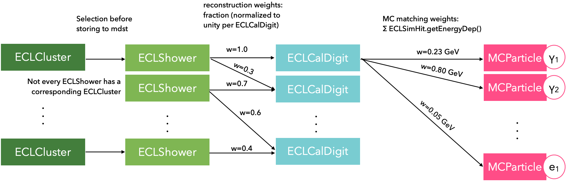
Fig. 7.1 Schematic diagram showing the weighted relations between ECL reconstruction objects and simulated particles.#
The overall weight for the relation between an ECLCluster object and a MCParticle is then given by the product of the weight between the corresponding ECLShower and ECLCalDigit and the weight
between the ECLCalDigit and MCParticle. For example, the weight of the relation between the first ECLCluster in Fig. 7.1 and MCParticle \(\gamma_2\) is given by \(1.0\times 0.8=0.8\) GeV.
When then a neutral Particle is reconstructed from a ECLCluster (so there is no reconstructed track matched to the cluster), it will be MCMatched in the modular analysis if the following conditions are true:
\(\mathrm{weight}/{E_\mathrm{rec}} > 0.2\)
\(\mathrm{weight}/{E_\mathrm{true}} > 0.3\)
where \({E_\mathrm{rec}}\) is the reconstructed Energy of the ECLCluster, and \({E_\mathrm{true}}\) is the generated MCParticle energy.
The weight here refers to the relation with the largest weight.
This means that if multiple relations between a given ECLCluster and MCParticles exist, only the relation with the largest weight will be used, and the
corresponding MCParticle with this relation will be used to decide the MCMatching.
A photon match is made if mcErrors == 0 and the MCParticle has a mcPDG == 22. If the chosen MCParticle does not correspond to a true photon, then the mcErrors \(\neq\) 0 and no correct match will be made (even if
another one of the smaller-weighted relations for the particle is correct).
Information regarding these weights can be accessed on a user-analysis level using the following variables:
Note
These weight variables can be used to help isolate photons that originate from beam background processes. Such photons typically have a very low total weight.
This information has been extracted from this talk. More details about MC matching for photons can be found there and from the references therein.
7.7.8. Topology analysis#
This section provides some information on the interface, repositories, and
documents of TopoAna,
which is a generic tool for the event type analysis of inclusive MC samples in
high energy physics experiments,
and hence a powerful tool for analysts to investigate the signals and backgrounds
involved in their works.
TopoAna is an offline tool independent of basf2.
It can take the output root files of the Analysis module as
input.
The MC truth information for the event type analysis can be stored in the root
files with the utility MCGenTopo in basf2.
Thus, MCGenTopo is the interface of basf2 to TopoAna.
Note
Apart from the interface, this section only introduces the TopoAna
resources outside the Belle II software documentation.
Inside the documentation, please see Section 3.5.6 for the
online textbook on TopoAna.
It is a good idea to start learning the usage of TopoAna with this online
textbook.
Please feel free to contact Xingyu Zhou (zhouxy@buaa.edu.cn) if you have any
questions or comments on TopoAna.
The interface#
As we mention above, MCGenTopo is the interface of basf2 to TopoAna.
To be specific, the interface implements the following parameter function
mc_gen_topo(n) in the script variables/MCGenTopo.py.
- variables.MCGenTopo.mc_gen_topo(n=200)[source]
Gets the list of variables containing the raw topology information of MC generated events. To be specific, the list including the following variables:
nMCGen: number of MC generated particles in a given event,MCGenPDG_i(i=0, 1, … n-2, n-1): PDG code of the \({\rm i}^{\rm th}\) MC generated particle in a given event,MCGenMothIndex_i(i=0, 1, … n-2, n-1): mother index of the \({\rm i}^{\rm th}\) MC generated particle in a given event.
Tip
Internally,
nMCGen,MCGenPDG_iandMCGenMothIndex_iare just aliases ofnMCParticles,genParticle(i, varForMCGen(PDG))andgenParticle(i, varForMCGen(mcMother(mdstIndex))), respectively.For more details on the variables, please refer to the documentations of
nMCParticles,genParticle,varForMCGen,PDG,mcMother, andmdstIndex.
- Parameters:
n (int) – number of
MCGenPDG_i/MCGenMothIndex_ivariables. Its default value is 200.
Note
To completely examine the topology information of the events in an MC sample, the parameter
nshould be greater than or equal to the maximum ofnMCGenin the sample.Normally, the maximum of
nMCGenin the MC samples at Belle II is less than 200. Hence, if you have no idea about the maximum ofnMCGenin your own MC sample, it is usually a safe choice to use the default parameter value 200.However, an overlarge parameter value leads to unnecessary waste of disk space and redundant variables with inelegant
nanvalues. Hence, if you know the maximum ofnMCGenin your own MC sample, it is a better choice to assign the parameter a proper value.
Below are the steps to use mc_gen_topo(n) to get the input data to TopoAna.
Append the following statement at the beginning part of your python steering script
from variables.MCGenTopo import mc_gen_topo
Use the parameter function
mc_gen_topo(n)as a list of variables in the steering functionvariablesToNtupleas followvariablesToNtuple(particleList, yourOwnVariableList + mc_gen_topo(n), treeName, fieName, path)
Run your python steering script with
basf2
Repositories#
The following three remote repositories of TopoAna are provided at present.
The one at DESY’s GitLab is most convenient to Belle II users.
Nonetheless, the two at GitHub and at GitLab of IHEP are also provided as helpful
alternatives for possible convenience.
Documents#
See also
The introduction to the documents can also be found in the file README.md
in the TopoAna package, which should be the first document to be read on
TopoAna.
For your convenience, a pdf and a html version of the README file are provided
in the TopoAna package as share/README.pdf and share/README.html,
respectively.
The following three documents of TopoAna are provided in its package.
A brief description of the tool is in the document:
share/quick-start_
tutorial_v*_Belle_II.pdf
All the examples in the quick-start tutorial can be found in the sub-directory
examples/in_the_quick-start_tutorial
A detailed description of the tool is in the document:
share/user_guide
_v*.pdf
All the examples in the user guide can be found in the sub-directory
examples/in_the_user_guide
An essential description of the tool is in the document:
share/paper_draft_v*.pdfAll the examples in the paper draft can be found in the sub-directory
examples/in_the_paper
Note
The paper on the tool has been published by
Computer Physics
Communications
. You can find this paper and the preprint corresponding to it in the links Comput. Phys. Commun. 258 (2021) 107540 and arXiv:2001.04016, respectively. If the tool really helps your researches, we would appreciate it very much if you could cite the paper in your publications.
As for the three documents, the quick-start tutorial is the briefest, the user guide is the most detailed, and the paper draft is composed of the essential and representative parts of the user guide.
Tip
It is a good practice to learn how to use the tool via the examples in the quick-start tutorial, user guide, and paper draft, in addition to the online textbook in Section 3.5.6.
Use cases at Belle II#
At the end of this section, we list two use cases of TopoAna at Belle II:
one for semitauonic analyses and the other for charm analyses.
You can refer to them if you work in the related analysis groups.
Using TopoAna with the semitauonic framework by Hannah Marie Wakeling
TopoAna Wrapper for Charm Analysis by Guanda Gong