20.2. SVD Offline Calibration
Here we briefly describe the so-called offline calibrations.
20.2.1. Hit Time Calibration
The time calibration is implemented in the Calibration Framework (CAF) and is run on 6-sample data with AirFlow.
The hit time calibration exploits the correlation between the time of the event EventT0 and the hit time. We select clusters associated to tracks and neglect the flight time of the particle.
For all three time estimators CoG6, CoG3 and ELS3 we first compute the time of the event in the SVD reference frame, \(t_0^{\rm SVD}\):
where \(\Delta t \simeq 31.44\) ns is the sampling period of the APV readout chip, \(TB = 0,1,2,3\) is the TriggerBin and provides the correct time shift to move into the SVD reference frame, and \(FF=0,1,2,3\) (FirstFrame) is applied only for CoG3 and ELS3 due to the MaxSum algorithm.
We build the 2D plot of the raw hit time \(t_{\rm raw}\) vs \(t_0^{\rm SVD}\). Note that the \(t_{\rm raw}\) is different for the three estimator.
We then take the ProfileX of the 2D plot and fit the correlation with a function that depends on the estimator. An example of correlation plot for CoG6, with calibration function superimposed is shown in the following figure:
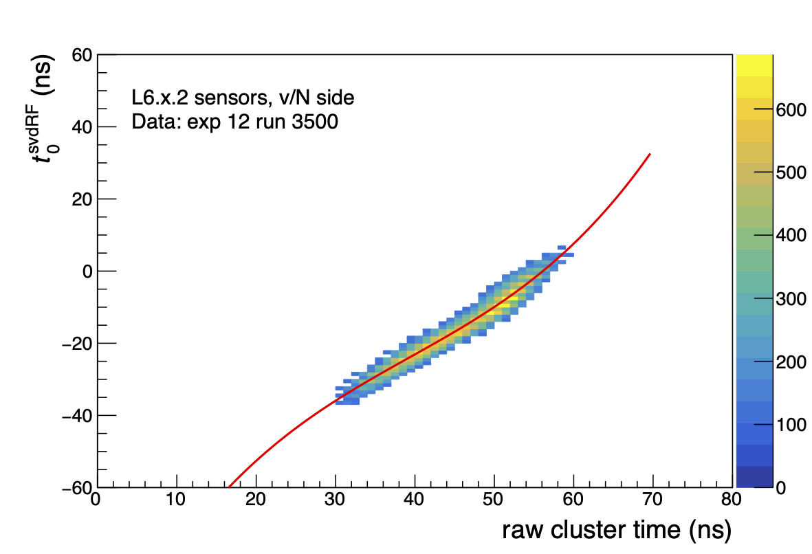
CoG6 Calibration Function
For CoG6 we use a third order polynomial:
CoG3 Calibration Function
For CoG3 we use a third order polynomial, but with a different parameterization:
ELS3 Calibration Function
For ELS3 we use the following calibration function: