6.7.5. Full event interpretation¶

Sphinx documentation¶

Algorithm overview¶

Physics¶

Measurements of decays including neutrinos, in particular rare decays, suffer from missing kinematic information. The FEI recovers this information partially and infers strong constraints on the signal candidates by automatically reconstructing the rest of the event in thousands of exclusive decay channels. The Full Event Interpretation (FEI) is an essential component in a wide range of important analyses, including: the measurement of the CKM element $|V_{ub}|$ through the semileptonic decay $b \rightarrow u \nu$; the search for a charged-Higgs effect in $B \rightarrow D \tau \nu$; and the precise measurement of the branching fraction of $B \rightarrow \tau \nu$, which is sensitive to new physics effects.

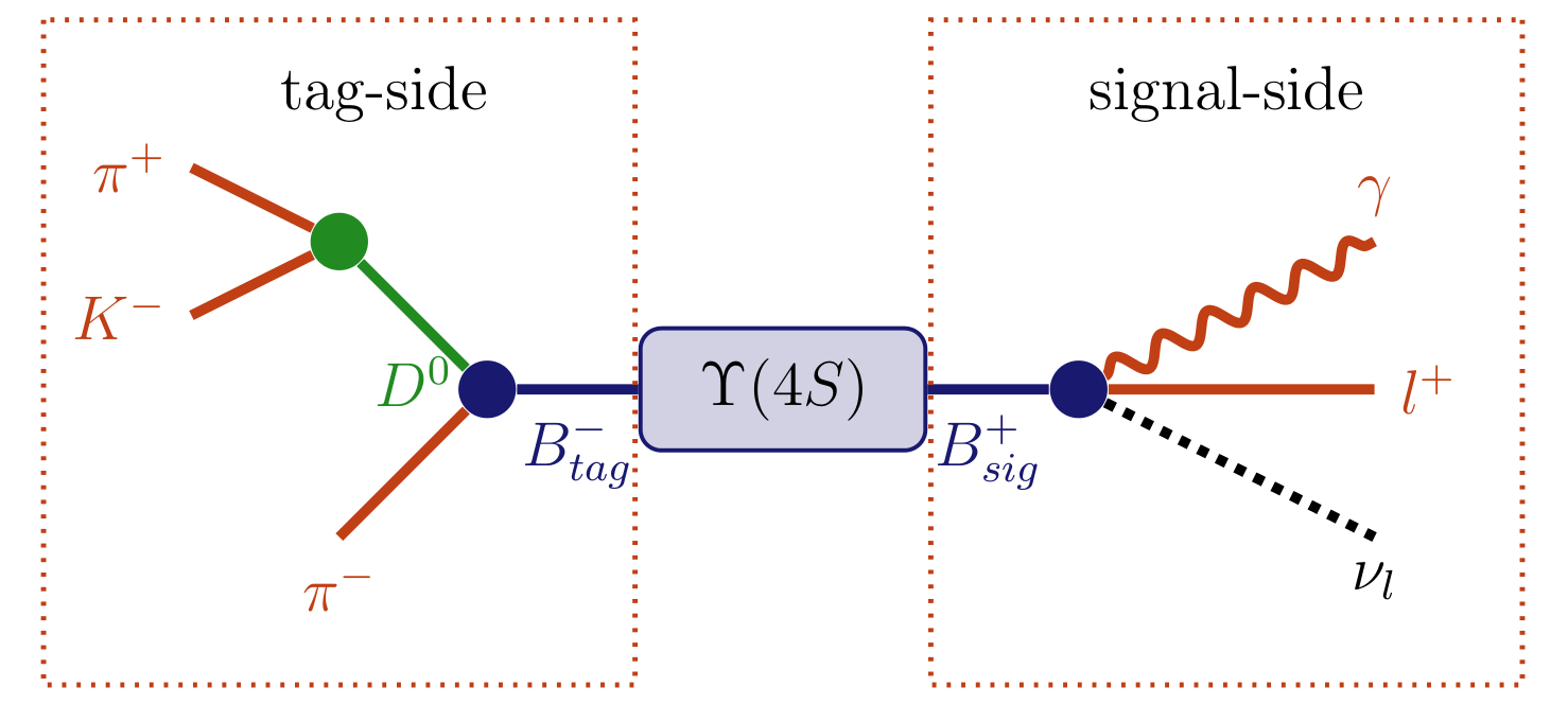
Fig. 6.8 $\Upsilon(4S)\rightarrow (B^{+} \rightarrow l^{+} \nu_{l} \gamma) (B^{-} \rightarrow (D^{0} \rightarrow K^{-} \pi^{+}) \pi^{-})$ decay topology. Here the decay $B^{-} \rightarrow (D^{0} \rightarrow K^{-} \pi^{+}) \pi^{-}$ can be reconstructed as the tag-side allowing additional information about the signal-side $B^{+} \rightarrow l^{+} \nu_{l} \gamma$ to be deduced.¶

As an analysis technique unique to B factories, the Full Event Interpretation will play an important role in the measurement of rare decays. This technique reconstructs one of the B mesons and infers strong constraints for the remaining B meson in the event using the precisely known initial state of the $\Upsilon(4S)$. The actual analysis is then performed on the second B meson. The two mesons are called tag-side $B_{\text{tag}}$ and signal-side $B_{\text{sig}}$, respectively. In effect the FEI allows one to reconstruct the initial $\Upsilon(4S)$ resonance, and thereby recovering the kinematic and flavour information of $B_{\text{sig}}$. Furthermore, the background can be drastically reduced by discarding $\Upsilon(4S)$ candidates with remaining tracks or energy clusters in the rest of event.

Belle already employed a similar technique called Full Reconstruction (FR) with great success. As a further development the Full Event Interpretation is more inclusive, provides more automation and analysis-specific optimisations. Both techniques heavily rely on multivariate classifiers (MVC). MVCs have to be trained on a Monte Carlo (MC) simulated data sample. However, the analysis-specific signal-side selection strongly influences the background distributions on the tag-side. Yet this influence had to be neglected by the FR, because the training of the MVCs was done independently from the signal-side analysis. In contrast, the FEI can be trained for each analysis separately and can thereby take the signal-side selection into account. The analysis-specific training is possible due to the deployment of speed-optimized training algorithms, full automation and the extensive usage of parallelization on all levels. The total training duration for a typical analysis is in the order of days instead of weeks. In consequence, it is also feasible to retrain the FEI if better MC data or optimized MVCs become available.

Key Performance Indicators¶

Quantifying the performance of the FEI can be done using:

the tagging efficiency, that is the fraction of $\Upsilon(4S)$ events which can be tagged,
the tag-side efficiency, that is the fraction of $\Upsilon(4S)$ events with a correct tag,
and the purity, that is the fraction of the tagged $\Upsilon(4S)$ events with a correct tag-side

These three properties are the key performance indicators used, they are closely related to important properties of a specific analysis: The tagging efficiency is important to judge the disk-space required for skimming; the tag-side efficiency influences the effective statistics of the analysis, and the purity is related to the signal-to-noise ratio of the analysis.

The tag-side efficiency and purity are usually shown in form of a receiver operating characteristic curve parametrized with the SignalProbability.

Hadronic, Semileptonic and Inclusive Tagging¶

As previously described, the FEI automatically reconstructs one out of the two $B$ mesons in an Υ(4S) decay to recover information about the remaining $B$ meson. In fact, there is an entire class of analysis methods, so-called tagging-methods, based on this concept. In the past there were three distinct tagging-methods: hadronic, semileptonic and inclusive tagging.

Hadronic tagging solely uses hadronic decay channels for the reconstruction. Hence, the kinematics of the reconstructed candidates are well known and the tagged sample is very pure. Then again, hadronic tagging is only possible for a tiny fraction of the dataset on the order of a few per mille.
Semileptonic tagging uses semileptonic $B$ decays. Due to the high branching fraction of semileptonic decays this approach usually has a higher tagging and tag-side efficiency. On the other hand, the semileptonic reconstruction suffers from missing kinematic information due to the neutrino in the final state of the decay. Hence, the sample is not as pure as in the hadronic case.
Inclusive tagging combines the four-momenta of all particles in the rest of the event of the signal-side $B$ candidate. The achieved tagging efficiency is usually one order of magnitude above the hadronic and semileptonic tagging. Yet the decay topology is not explicitly reconstructed and cannot be used to discard wrong candidates. In consequence, the methods suffers from a high background and the tagged sample is very impure.

The FEI combines the first two tagging-methods: hadronic and semileptonic tagging, into a single algorithm. Simultaneously it increases the tag-side efficiency by reconstructing more decay channels in total. The long-term goal is to unify all three methods in the FEI. The algorithm presented in this thesis is only the first step in this direction.

Hierarchical Approach¶

The basic idea of the Full Event Interpretation is to reconstruct the particles and train the MVCs in a hierarchical approach. At first the final-state particle candidates are selected and corresponding classification methods are trained using the detector information. Building on this, intermediate particle candidates are reconstructed and a multivariate classifier is trained for each employed decay channel. The MVC combines all information about a candidate into a single value – the signal-probability. In consequence, candidates from different decay channels can be treated equally in the following reconstruction steps.

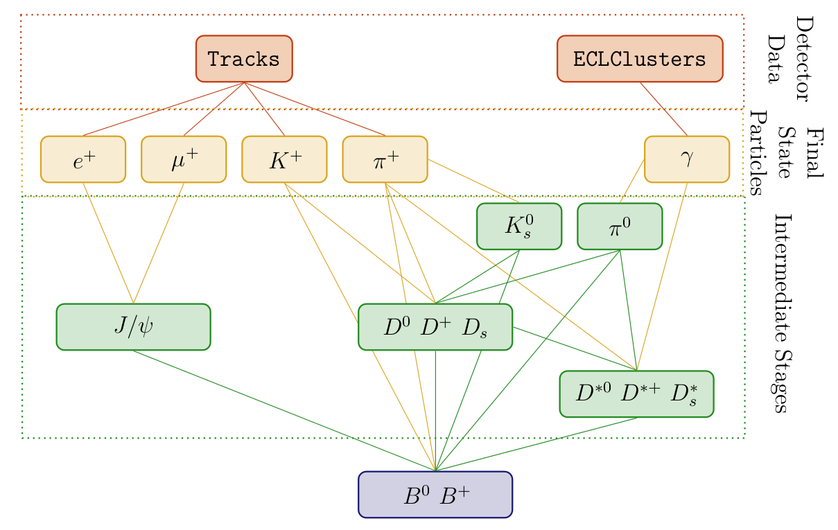
Fig. 6.9 Hierarchical reconstruction applied by the FEI, which starting from tracks and EM clusters reconstructs initial state particles, intermediate particles in several stages and finally candidate $B$ tags.¶

For instance, the FEI currently reconstructs 15 decay channels of the $D^{0}$ . Afterwards, the generated D0 candidates are used to reconstruct $D^{*0}$ in 2 decay channels. All information about the specific D0 decay channel of the candidate is encoded in its signal-probability, which is available to the $D^{*0}$ classifiers. In effect, the hierarchical approach reconstructs $2 * 15 = 30$ exclusive decay channels and provides a signal-probability for each candidate, which makes use of all available information. Finally, the $B$ candidates are reconstructed and the corresponding classifiers are trained. The final output of the FEI to the user contains four ParticleLists: B+:hadronic, B+:semileptonic, B0:hadronic and B0:semileptonic.

It is important to introduce intermediate cuts to reduce combinatorics in order to save computation time. The main goal of the cuts is to limit the combinatoric, while retaining the best $B$ meson candidates in each event. There are two types of cuts

PreCuts can be chosen for each channel individually and are done as early in the reconstruction as possible to save computing time.
PostCuts are applied after all information about the candidate from the vertex fitting and the MVC is available; The post-cut employs all available information about a candidate by cutting on the signal-probability calculated by the MVC. Since the interpretation of the signal probability is the same for all candidates independent of their decay channels the cut is channel-independent. It is important to choose this cut tight enough, otherwise one loses a lot of signal candidates in the consecutive reconstruction steps due to a bad signal-to-noise ratio

The FEI uses several cuts, which are applied for each particle in the following order:

PreCut::userCut is applied before all other cuts to introduce a-priori knowledge, e.g. final-state particle tracks (K shorts are handled via V0 objects) should originate from the IP '[dr < 2] and [abs(dz) < 4]', the invariant mass of D mesons should be inside a certain mass window '1.7 < M < 1.95', hadronic B meson candidates require a reasonable beam-constrained mass and delta E 'Mbc > 5.2 and abs(deltaE) < 0.5'. This cut is also used to enforce constraints on the number of additional tracks in the event for a specific signal-side 'nRemainingTracksInEvent == 1'.
PreCut::bestCandidateCut keeps for each decay-channel only a certain number of best-candidates. The variable which is used to rank all the candidates in an event is usually the PID for final-state particles e.g. electronID, pionID, muonID`; the distance to the nominal invariant mass abs(dM) for intermediate particles; the product of the daughter SignalProbabilities for intermediate particles in semileptonic or KLong channels daughterProductOf(extraInfo(SignalProbability)). Between 10-20 candidates per channel (charge conjugated candidates are counted separately) are typically kept at this stage. This reduces the combinatoric in each event to the same level.
PreCut::vertexCut throws away candidates below a certain confidence level after the vertex fit. Default is throwing away only candidates with failed fits. Since the vertex fit is the most expensive part of the reconstruction it does not make sense to do a harder cut here, because the cuts on the network output afterwards will be more efficient without to much extra computing time
PostCut::value is a cut on the absolute value of the SignalProbability and should be chosen very loose, only candidates which are highly unlikely should be thrown away here
PostCut::bestCandidateCut keeps for each particle only a certain number of best-candidates. The candidates of all channels are ranked using their SignalProbability. Usually Between 10-20 candidates are kept per particle. This cut is extremely important because it limits the combinatoric in the next stage of reconstructions, and the algorithm can calculate the combinatoric at the next stage in advance.

Applying the FEI¶

Just include the feistate.path created by the fei.get_path() function in your steering file.

The weightfiles are automatically loaded from the conditions database (see FEI and the conditions database). This might take some time.

After the FEI path the following lists are available

B+:generic (hadronic tag)
B+:semileptonic (semileptonic tag)
B0:generic (hadronic tag)
B+:semileptonic (semileptonic tag)

Each candidate has two extra infos which are interesting:

SignalProbability is the signal probability calculated using FastBDT
decayModeID is the tag $B$ decay channel

You can use a different decay channel configuration during the application. In particular you can omit decay channels (e.g. the semileptonic ones if you are only interested in the hadronic tag). However, it is not possible to add new channels without training them first (obviously).

You can find up to date examples in analysis/examples/FEI. If you encounter problems which require debugging in the FEI algorithm, the best starting point is to enable the monitoring, by choosing monitor=True in the FEIConfiguration. This will create a lot of root files containing histograms of interesting variables throughout the process (e.g. MC truth before and after all the cuts). You can also create a pdf using the root files produced by the monitoring and the “Summary.pickle” file produced by the original training by executing:

basf2 fei/latexReporting.py > summary.tex

FEI and the conditions database¶

The FEI is frequently retrained and updated to give the best performance with the latest reconstruction, etc. You will need to use the relevant database in which the FEI training weights are located. FEI training weights are distributed by the basf2.conditions database under an analysis global tag. In order to find the latest, recommended FEI training, you can use the b2conditionsdb-recommend: Recommend a global tag to analyse a given file tool.

b2conditionsdb-recommend input_file.mdst.root

This tool will tell you all tags you should use. For the FEI we are only concerned with the analysis tag. Analysis tags are named analysis_tools_XXXX, and the latest and recommended one can be retrieved using the function modularAnalysis.getAnalysisGlobaltag(). You will need to prepend this tag to your global tags list. This is done inside the FEI steering script.

import basf2
import fei

basf2.conditions.prepend_globaltag("analysis_tools_XXXX")
conf = fei.config.FeiConfiguration(prefix="foo", ...)

Note that when running on Belle converted data or MC you will need to use the B2BII and B2BII_MC database tags, respectively.

If you have trouble finding the correct analysis tag, please ask a question at B2Questions and/or send a mail to frank.meier@belle2.org,

Sphinx documentation¶

Full Event Interpretation framework for Belle II Thomas Keck, Christian Pulvermacher 2013-2017

Detailed usage examples can be found in analysis/examples/FEI/

class fei.FeiState(path, stage, plists)¶

property path¶: Alias for field number 0

property plists¶: Alias for field number 2

property stage¶: Alias for field number 1

fei.get_path(particles: Sequence[fei.config.Particle], configuration: fei.config.FeiConfiguration) → fei.core.FeiState[source]¶

The most important function of the FEI. This creates the FEI path for training/fitting (both terms are equal), and application/inference (both terms are equal). The whole FEI is defined by the particles which are reconstructed (see default_channels.py) and the configuration (see config.py).

TRAINING For training this function is called multiple times, each time the FEI reconstructs one more stage in the hierarchical structure i.e. we start with FSP, pi0, KS_0, D, D*, and with B mesons. You have to set configuration.training to True for training mode. All weight files created during the training will be stored in your local database. If you want to use the FEI training everywhere without copying this database by hand, you have to upload your local database to the central database first (see documentation for the Belle2 Condition Database).

APPLICATION For application you call this function once, and it returns the whole path which will reconstruct B mesons with an associated signal probability. You have to set configuration.training to False for application mode.

MONITORING You can always turn on the monitoring (configuration.monitor = True), to write out ROOT Histograms of many quantities for each stage, using these histograms you can use the printReporting.py or latexReporting.py scripts to automatically create pdf files.

LEGACY This function can also use old FEI trainings (version 3), just pass the Summary.pickle file of the old training, and the weight files will be automatically converted to the new naming scheme.

Parameters

particles – list of config.Particle objects
config – config.FeiConfiguration object

fei.get_default_channels(B_extra_cut=None, hadronic=True, semileptonic=True, KLong=False, baryonic=True, chargedB=True, neutralB=True, specific=False, removeSLD=False)[source]¶

returns list of Particle objects with all default channels for running FEI on Upsilon(4S). For a training with analysis-specific signal selection, adding a cut on nRemainingTracksInRestOfEvent is recommended.

Parameters

B_extra_cut – Additional user cut on recombination of tag-B-mesons
hadronic – whether to include hadronic B decays (default is True)
semileptonic – whether to include semileptonic B decays (default is True)
KLong – whether to include K_long decays into the training (default is False)
baryonic – whether to include baryons into the training (default is True)
chargedB – whether to recombine charged B mesons (default is True)
neutralB – whether to recombine neutral B mesons (default is True)
specific – if True, this adds isInRestOfEvent cut to all FSP
removeSLD – if True, removes semileptonic D modes from semileptonic B lists (default is False)

fei.get_unittest_channels(specific=False)[source]¶

fei.do_trainings(particles: Sequence[fei.config.Particle], configuration: fei.config.FeiConfiguration)[source]¶

Performs the training of mva classifiers for all available training data, this function must be either called by the user after each stage of the FEI during training, or (more likely) is called by the distributed.py script after merging the outputs of all jobs,

Parameters

particles – list of config.Particle objects
config – config.FeiConfiguration object

Returns

list of tuple with weight file on disk and identifier in database for all trained classifiers

class fei.Particle(identifier: str, mvaConfig: fei.config.MVAConfiguration, preCutConfig: fei.config.PreCutConfiguration = PreCutConfiguration(userCut='', vertexCut=- 2, noBackgroundSampling=False, bestCandidateVariable=None, bestCandidateCut=0, bestCandidateMode='lowest'), postCutConfig: fei.config.PostCutConfiguration = PostCutConfiguration(value=0.0, bestCandidateCut=0))[source]¶

The Particle class is the only class the end-user gets into contact with. The user creates an instance of this class for every particle he wants to reconstruct with the FEI algorithm, and provides MVAConfiguration, PreCutConfiguration and PostCutConfiguration. These can be overwritten per channel.

addChannel(daughters: Sequence[str], mvaConfig: fei.config.MVAConfiguration = None, preCutConfig: fei.config.PreCutConfiguration = None)[source]¶

Appends a new decay channel to the Particle object.

Parameters

daughters – is a list of pdg particle names e.g. [‘pi+’,’K-‘]
mvaConfig – multivariate analysis configuration
preCutConfig – pre cut configuration object

channels = None¶: DecayChannel objects added by addChannel() method.

property daughters¶: Property returning list of unique daughter particles of all channels

identifier = None¶: pdg name of the particle with an optional additional user label separated by:

label = None¶: Additional label like hasMissing or has2Daughters

mvaConfig = None¶: multivariate analysis configuration (see MVAConfiguration)

name = None¶: The name of the particle as correct pdg name e.g. K+, pi-, D*0.

postCutConfig = None¶: post cut configuration (see PostCutConfiguration)

preCutConfig = None¶: intermediate cut configuration (see PreCutConfiguration)

class fei.MVAConfiguration¶

Multivariate analysis configuration class.

property config¶: Method specific configuration string passed to basf2_mva_teacher

property method¶: Method used by MVAInterface.

property sPlotVariable¶: Discriminating variable used by sPlot to do data-driven training.

property target¶: Target variable from the VariableManager.

property variables¶: List of variables from the VariableManager.{} is expanded to one variable per daughter particle.

class fei.PreCutConfiguration¶

PreCut configuration class. These cuts is employed before training the mva classifier.

property bestCandidateCut¶: Number of best-candidates to keep after the best-candidate ranking.

property bestCandidateMode¶: Either lowest or highest.

property bestCandidateVariable¶: Variable from the VariableManager which is used to rank all candidates.

property noBackgroundSampling¶: For very pure channels, the background sampling factor is too high and the MVA can’t be trained. This disables background sampling.

property userCut¶: The user cut is passed directly to the ParticleCombiner.Particles which do not pass this cut are immediately discarded.

property vertexCut¶: The vertex cut is passed as confidence level to the VertexFitter.

class fei.PostCutConfiguration¶

PostCut configuration class. This cut is employed after the training of the mva classifier.

property bestCandidateCut¶: Number of best-candidates to keep, ranked by SignalProbability.

property value¶: Absolute value used to cut on the SignalProbability of each candidate.

class fei.FeiConfiguration¶

Fei Global Configuration class

property cache¶: The stage which is passed as input, it is assumed that all previous stagesdo not have to be reconstructed again. Can be either a number or a filename containing a pickled number or None in this case the environment variable FEI_STAGE is used.

property externTeacher¶: Teacher command e.g. basf2_mva_teacher, externClusterTeacher

property legacy¶: Pass the summary file of a legacy FEI training,and the algorithm will be able to apply this training.

property monitor¶: If true, monitor histograms are created

property prefix¶: The database prefix used for all weight files

property training¶: If you train the FEI set this to True, otherwise to False

class fei.DecayChannel¶

Decay channel of a Particle.

property daughters¶: List of daughter particles of the decay channel e.g. [K+, pi-]

property decayModeID¶: DecayModeID of this channel. Unique ID for each channel of this particle.

property decayString¶: DecayDescriptor of the channel e.g. D0 -> K+ pi-

property label¶: Label used to identify the decay channel e.g. for weight files independent of decayModeID

property mvaConfig¶: MVAConfiguration object which is used for this channel.

property name¶

Name of the channel e.g. D0:generic_0

Type: str

property preCutConfig¶: PreCutConfiguration object which is used for this channel.

Code structure¶

In my opinion the best way to use and learn about the FEI is to read the code itself. I wrote an extensive documentation. Hence I describe here the code structure. If you don’t want to read code, you can just skip this part.

The FEI is completely written in Python and does only use general purpose BASF2 modules. You can find the code under: analysis/scripts/fei/

config.py¶

The classes defined here are used to uniquely define a FEI training.

The global configuration like database prefix, cache mode, monitoring, … (FeiConfiguration)
The reconstructed Particles (Particle)
The reconstructed Channels of each particle (DecayChannel)
The MVA configuration for each channel (MVAConfiguration)
The Cut definitions of each channel (PreCutConfiguration)
The Cut definitions of each particle (PostCutConfiguration)

These classes are used to define the default configuration of the FEI

default_channels.py¶

Contains some example configurations of the FEI. Mostly you want to use get_default_channels(), which can return the configuration for common use-cases

Hadronic tagging (hadronic = True)
Semileptonic tagging (semileptonic = True)
B+/B- (chargedB = True)
B0/anti-B0 (neutralB = True)
running on Belle 1 MC/data (convertedFromBelle = True)
running a specific FEI which is optimized for a signal selection and uses ROEs (specific = True)

You can turn on and off individual parts of the reconstruction. I advise to train with the all parts, and then turn off the parts you don’t need in the application.

Another interesting configuration is given by get_fr_channels, which will return a configuration which is equivalent to the original Full Reconstruction algorithm used by Belle

Keep in mind, you can write your own configuration. E.g. for $B_{s}$ particles

In the training and application steering file you probably will use:

import fei
particles = fei.get_default_channels(hadronic=True, semileptonic=True, chargedB=True, neutralB=True)

core.py¶

This file contains the implementation of the Full Event Interpretation Algorithm.

Some basic facts:

The algorithm will automatically reconstruct $B$ mesons and calculate a signal probability for each candidate.
It can be used for hadronic and semileptonic tagging.
The algorithm has to be trained on MC, and can afterwards be applied on data.
The training requires O(100) million MC events
The weightfiles are stored in the Belle 2 Condition database

Read this file if you want to understand the technical details of the FEI.

The FEI follows a hierarchical approach.

There are 7 stages:

(Stage -1: Write out information about the provided data sample)
Stage 0: Final State Particles (FSP)
Stage 1: $pi^{0}$, $J/\psi$ (and $Lambda^{0}$ if baryonic modes requested)
Stage 2: $K_{s}$ (and $Sigma^{+}$ if baryonic modes requested)
Stage 3: $D$ mesons (and $Lambda_{c}^{+}$ if baryonic modes requested)
Stage 4: $D^{*}$ mesons
Stage 5: $B$ mesons
Stage 6: Finish

Most stages consists of:

Create Particle Candidates
Apply Cuts
Do vertex Fitting
Apply a multivariate classification method
Apply more Cuts

The FEI will reconstruct these 7 stages during the training phase, since the stages depend on one another, you have to run basf2 multiple (7) times on the same data to train all the necessary multivariate classifiers.

Since running a 7-phase training by hand would be very difficult there is a tool which implements the training (including distributing the jobs on a cluster, merging the training files, running the training, …)

Training the FEI¶

The FEI has to be trained on Monte Carlo data and is applied subsequently on real data after an analysis-specific signal-side selection. There are three different types of events one has to consider in the training and application of the FEI:

double-generic events - $e^{+}e^{-} \rightarrow \Upsilon(4S)\rightarrow B \bar{B}$ for charged and neutral B pairs, where both B mesons decay generically.
continuum events - $e^{+}e^{-} \rightarrow \Upsilon(4S)\rightarrow q \bar{q}$ where $q=u,d,s,c$.
and signal events - $e^{+}e^{-} \rightarrow \Upsilon(4S)\rightarrow B \bar{B}$, where one $B$ decays generically and the other decays in an analysis-specific signal-channel like $B^{+} \rightarrow \tau^{+} \nu_{\tau}$.

The final classifier output for the B tag mesons has to identify correctly reconstructed B tag mesons in the signal events of the analysis and reject background B tag mesons from double-generic, continuum and signal events efficiently. To accomplish a high efficiency for correctly reconstructed B tag in signal events a training on pure signal Monte Carlo after the signal-side selection would be appropriate, but in this scenario background components from double-generic and continuum events would not be considered in the training and therefore could not be rejected efficiently. On the other hand, a training on double-generic and continuum Monte Carlo after signal-side selection suffers from low statistics especially for correctly reconstructed B tag mesons, because the constraint that the reconstructed candidate has to use all remaining tracks is very strict. Moreover, it is not clear if D mesons from continuum background should be considered as signal in the corresponding trainings.

The background components are factorized into background from Υ(4S) decays and from continuum events. It is assumed that the continuum events can be suppressed efficiently with the ContinuumSuppression module, therefore no Monte Carlo data for continuum events is used in the training of the FEI. Further studies have to be performed to test this assumption.

The FR of Belle was trained on double-generic and continuum Monte Carlo without considering the signal-side selection. In consequence, the background distributions were fundamentally different in training and application. For example, most of the CPU time in the training was used for events with more than 12 tracks, yet these events never led to a valid $B$ tag meson in an analysis with only one track on the signal-side like $B^{+} \rightarrow \tau^{+} \nu_{\tau}$. Therefore the FEI employs two different training modes:

generic-mode; the training is done on double-generic Monte Carlo without signal-side selection, which corresponds to the FR of Belle. Hence, the training is independent of the signal-side and is only trained once for all analyses. The method is optimized to reconstruct tag-side of generic MC. If you don’t know your signal-side selection before the tag-side is reconstructed e.g. in an inclusive analysis like $B → X_c K$ or $B → X_{u/c} l \nu$, this is the mode you want.
specific-mode; the training is optimized for the signal-side selection and trained on double-generic and signal Monte Carlo, in order to get enough signal statistics despite the no-remaining-tracks constraint. In this mode the FEI is trained on the RestOfEvent after the signal-side selection, therefore the training depends on the signal-side and one has to train it for every analysis separately. The method is optimized to reconstruct the tag-side of signal MC. The usual tag-side efficiency is no longer a good measure for the quality, instead you have to look at the total Y4S efficiency including your signal-side efficiency. This mode can be used in searches for $B^{+} \rightarrow \tau^{+} \nu_{\tau}$ (Thomas Keck), $B^{+} \rightarrow l^{+} \nu_{l} \gamma$ (Moritz Gelb), $B^{0} \rightarrow \nu \bar{\nu}$ (Gianluca Inguglia), $B \rightarrow K^{*} \nu \bar{\nu}$, $B \rightarrow D^{*} \tau \nu_{\tau}$, … Another advantage is that global constraints on the beam-constrained mass and $\Delta E$ can be enforced at the beginning of the training.

In addition it is possible to train the multivariate classifiers for an decay-channel on real data using sPlot, however I never tested it since we do not have real data (02/2016). We also trained the FEI successfully using Belle I MC. This is commonly known as “converted FEI”.

Basic Workflow (training)¶

If you want to use the FEI in your analysis these are the steps you have to do (italic font refers only to specific-mode):

Get an account on KEKCC or access to another cluster where you can submit computing jobs. You will need 10-20 TB disk space during the training (we cache the reconstructed training data to save a lot of computing time)! Once the training is done you only need O(100MB) of data.
Locate the generic Monte Carlo from the current MC campaign, you will need ~100M Events (the more the better). Generate 50M-100M Monte Carlo events with one B decaying into your signal-channel, the other B decaying generically.
Create a new directory and two subdirectories named “collection” and “jobs”
Copy an example steering file from analysis/examples/FEI/ to your directory and modify it (especially choose a different prefix(!))
Use python3 analysis/scripts/fei/distributed.py to perform the training
Take a look at the summary.pdf which is created at the end of the training
Upload the weightfiles to the condition database: b2conditionsdb-request localdb/database.txt
Load the path in your analysis-steering file by choosing the option training=False in the FEIConfiguration
Use the ParticleLists created by the FEI B+:generic, B+:semileptonic, B0:generic, B0:semileptonic and the signal-probabilities stored in the extra Info (extraInfo(SignalProbability)) in your analysis.

In addition you may want to train the ContinuumSuppression separately and use it.

A typical training of the generic FEI will take about a week on the new KEKCC cluster using 100 cores and 100M events. The specific FEI can be trained much faster, but will require more statistics depending on your signal side selection

distributed.py¶

This script can be used to train the FEI on a cluster like available at KEKCC. All you need is a basf2 steering file (see analysis/examples/FEI/ ) and some MC O(100) million

The script will automatically create some directories collection containing weightfiles, monitoring files and other stuff jobs containing temporary files during the training (can be deleted afterwards)

The distributed script automatically spawns jobs on the cluster (or local machine), and runs the steering file on the provided MC. Since a FEI training requires multiple runs over the same MC, it does so multiple times. The output of a run is passed as input to the next run (so your script has to use RootInput and RootOutput). In between it calls the do_trainings function of the FEI, to train the multivariate classifiers of the FEI at each stage. At the end it produces summary outputs using printReporting.py and latexReporting.py (this will only work of you use the monitoring mode). And a summary file for each mva training using basf2_mva_evaluate. If your training fails for some reason (e.g. a job fails on the cluster), the FEI will stop, you can fix the problem and resume the training using the -x option. This requires some expert knowledge, because you have to know how to fix the occurred problem and at which step you have to resume the training. After the training the weightfiles will be stored in the localdb in the collection directory. You have to upload these local database to the Belle 2 Condition Database if you want to use the FEI everywhere. Alternatively you can just copy the localdb to somewhere and use it directly, however, this is recommended only for testing as it is not reproducible.

You have to adjust the following parameters:

-n/--nJobs - the number of jobs which are submitted to the cluster. Every job has to process #input-files/nJobs data-files, so the number of jobs depend on the time-limit of each job on the cluster and the total number of files (assuming each file containing 1000 Events) you want to use for the training. On KEKCC nJobs=1000 for 100M Events (==100000 files) with a time limit of 3h on the short queue is sufficient.
-f/--steeringFile - the absolute path to the fei-training steering file.
-w/--workingDirectory - the absolute path to the working directory. This directory temporarily stores large training files, cut histograms, and other ntuples produced during the training of the FEI O(100GB).
-l/--largeDirectory - (optional) the absolute path to a directory with a lot of free space. The caching data O(10TB) is saved here, otherwise in the working directory.
-d/--data - The absolute paths to all your input files. You can use the bash glob expansion magic here (e.g. *)
-s/--site - The site you’re running on: At the moment kekcc, kitekp and local is supported.
-x/--skip-to - Skip to a specific step of the training. This is useful if you have to restart a training due to an earlier error (this is more an expert option).

Here’s a complete example:

python3 analysis/scripts/fei/distributed.py -s kekcc -f /home/belle2/tkeck/basf2/analysis/examples/FEI/B_generic.py -w /gpfs/fs02/belle2/users/tkeck/Belle2Generic_20160222 -n 1000 -d /ghi/fs01/belle2/bdata/MC/fab/merge/release-00-05-03/DBxxxxxxxx/MC5/prod00000013/s00/e0002/4S/r00001/mixed/sub00/\*.root -d /ghi/fs01/belle2/bdata/MC/fab/merge/release-00-05-03/DBxxxxxxxx/MC5/prod00000014/s00/e0002/4S/r00001/charged/sub00/\*.root

Known issues when training the FEI on the KEK system:

The automatic training can crash at several places. In most cases you hit a resource limit on your local machine or on your cluster

Disk space: Use df -h and du -sch to check this. Often this happens for directories that are not located at the HSM. E.g. the job directory due to large log files, or collection directory due to a large training file
Total number of processes: The FEI doesn’t use that much processes, still you can run into problems at KEKCC if other users use the machine in parallel.
CPU time on cluster: Make sure that each job has enough cpu time to finish before it is killed by the cluster-software. If the job on the first stage takes 15 minutes, intermediate stages can take up to ten times more!

Restarting a training¶

If the training failed or you have to terminate a training temporarily you can usually restart it. The distributed script provides a option -x, which can restart the process at any point, and can even resubmit failed jobs.

I advise to take a look into the distributed.py script which is very well documented. Examples

You can find up to date examples in analysis/examples/FEI.

In general a FEI training steering file consists of

a decay channel configuration usually you can just use the default configuration in fei.get_default_channels. This configuration defines all the channels which should be reconstructed, the cuts, and the mva methods. You can write your own configuration, just take a look in analysis/scripts/fei/default_channels.py
a FeiConfiguration object, this defines the database prefix for the weightfiles and some other things which influence the training (e.g. if you want to run with the monitoring, or if you use b2bii)
a feistate object, which contains the BASF2 path for the current stage, you get this with the get_path function

The user is responsible for writing the input and output part of the steering file. Depending on the training mode (generic / specific) this part is different for each training (see below for examples). The FEI algorithm itself just assumes that the DataStore already contains a valid reconstructed event, and starts to reconstruct B mesons. During the training the steering file is executed multiple times. The first time it is called with the Monte Carlo files you provided, and the complete DataStore is written out at the end. The following calls must receive the previous output as input.

You can find up to date examples for training the specific or generic FEI, for the cases of Belle II of Belle converted data / MC in analysis/examples/FEI.

Applying the FEI¶

Just include the feistate.path create by the fei.get_path() function in your steering file.

The weightfiles are automatically loaded from the condition database. This might take some time. You can also copy the localdb of the training (or another local database containing the weightfiles) in your working directory by hand to speed up the execution.

After the FEI path the following lists are available

B+:generic (hadronic tag)
B+:semileptonic (semileptonic tag)
B0:generic (hadronic tag)
B+:semileptonic (semileptonic tag)

Each candidate has three extra infos which are interesting:

SignalProbability is the signal probability calculated using FastBDT
decayModeID is the tag $B$ decay channel
uniqueSignal marks all unique candidates (because some Bs can be reconstructed in more than one decay channel

You can use a different decay channel configuration during the application. In particular you can omit decay-channels (e.g. the semileptonic if your are only interested in the hadronic tag). However, it is not possible to add new channels without training them first (obviously).

You can find up to date examples in analysis/examples/FEI. If you encounter problems which require debugging in the FEI algorithm, the best starting point is to enable the monitoring, by choosing monitor=True in the FEIConfiguration. This will create a lot of root files containing histograms of interesting variables throughout the process (e.g. MC truth before and after all the cuts). You can also create a pdf using the root files produced by the monitoring and the “Summary.pickle” file produced by the original training by executing:

basf2 fei/latexReporting.py > summary.tex

FEI and the condition database¶

The FEI is frequently retrained and updated to give the best performance with the latest reconstruction, etc. You will need to use the relevant database in which the FEI training weights are located. FEI training weights are distributed by the basf2.conditions database under an analysis global tag. In order to find the latest, recommended FEI training, you can use the b2conditionsdb-recommend: Recommend a global tag to analyse a given file tool.

b2conditionsdb-recommend input_file.mdst.root

This tool will tell you all tags you should use. For the FEI we are only concerned with the analysis tag. Analysis tags are named analysis_tools_XXXX. You will need to prepend this tag to your global tags list. This is done inside the FEI steering script.

import basf2
import fei

basf2.conditions.prepend_globaltag("analysis_tools_XXXX")
conf = fei.config.FeiConfiguration(prefix="foo", ...)

Note that when running on Belle converted data or MC you will need to use the B2BII and B2BII_MC database tags, respectively.

If you have trouble finding the correct analysis tag, please ask a question at B2Questions and/or send a mail to frank.meier@belle2.org,

Troubleshooting¶

Crash in the Neurobayes Library¶

The mva package NeuroBayes is used in the KShort Finder of the belle software. However, NeuroBayes is no longer officially supported by the company who developed it and also not by the Belle II collaboration. Nevertheless, you still need it to run b2bii.

There is a working neurobayes installation at KEKCC which you can use. This does mean that you can only use b2bii (and in consequence the FEI on converted MC) if you work on KEKCC.

If you are on KEKCC and get a crash you probably forgot to set the correct LD_LIBRARY_PATH

export LD_LIBRARY_PATH=/sw/belle/local/neurobayes/lib/:$LD_LIBRARY_PATH

You have to set this AFTER you set up basf2, otherwise basf2 will override the LD_LIBRARY_PATH again.

Note that the NeuroBayes libraries which are shipped with the basf2 externals are only dummy libraries which are used during the linking of b2bii. They do not contain any NeuroBayes code, only functions with the correct signatures which will crash if they are called. Therefore it is important that the correct NeuroBayes libraries are found by the runtime-linker BEFORE the libraries shipped with basf2. This means you have to add the neurobayes path before the library path of the externals.

Running FEI on converted Belle MC outside of KEK¶

There are two problems with this:

You don’t have access to the old Belle condition database outside of KEK
You don’t have access to the NeuroBayes installation outside of KEK

To access the old Belle database anyway you have to forward to server to you local machine and set the environment variables correctly

ssh -L 5432:can01kc.cc.kek.jp:5432 tkeck@cw02.cc.kek.jp

export BELLE2_FILECATALOG=NONE

export USE_GRAND_REPROCESS_DATA=1

export PGUSER=g0db

export BELLE_POSTGRES_SERVER=localhost

Depending on how you use b2bii, the BELLE_POSTGRES_SERVER will be overridden by b2bii. Hence you have to enforce that localhost is used anyway. You can ensure this by adding:

import os

os.environ['BELLE_POSTGRES_SERVER'] = 'localhost'

directly before you call process().

The second problem is more difficult. You require a neurobayes installation. On KEKCC the installation is here /sw/belle/local/neurobayes/, and you might be tempted to copy the files from here and to run it on your local machine. However you require a license to run neurobayes on your machine. Since the latest neurobayes release 4.3.1 this license requirement is no longer technically enforced.

Neurobayes versions for Ubuntu (instead of SL6) are available as well.

Anyway don’t forget to add neurobayes to your LD_LIBRARY_PATH after(!) you set up basf2

export LD_LIBRARY_PATH=/sw/belle/local/neurobayes/lib/:$LD_LIBRARY_PATH

Btw, the Neurobayes libraries which are shipped with the basf2 externals are only dummy libraries which will just crash if you try to use them. They are only used so everybody can compile b2bii (because you require the libraries to link the b2bii modules).

Speeding up the FEI¶

The FEI is optimized for maximum speed, but the default configuration is not suitable for all applications. This means, one can save a lot of computing time. Here is a short list of things you can do to speed up the application of the FEI.

Use Fast Fit instead of KFit will gain a factor 2.
Deactivate the reconstruction unused B lists (by default hadronic, semileptonic, charged and neutral are all created) (see analysis/script/fei/default_channels.py). The get_default_channels function has parameters for this.
If you use the semileptonic tag but don’t want to use semileptonic D decays, you can deactivate them. But you have to comment out the corresponding channels in the get_default_channels function, or create your own custom channel configuration.
Add extra cuts before the combination of the B mesons, e.g. the cut on Mbc is by default for hadronic B mesons only >5.2. There is a parameter called B_extra_cut in the get_default_channels function.
Add a skim cut on the number of tracks. Just add an applyEventCuts to your path before running the FEI. In fact, the maximum number of tracks for a correct B candidate is 7 (not in theory, but in practice). Hence, If you know you only want one track on the signal side. You can discard all events with more than 8 tracks from the beginning, without losing any correctly reconstructed signal events. This is of course not possible for an inclusive signal-side.

With FEIv4 you don’t need to re-train anything if you apply the above mentioned changes. Deactivating channels and tightening cuts is fine. For instance, I made a large study on the influence of the track-cut described above, and it doesn’t matter at all if you use choose a different cut than the one used during the training.

Area for Future design and Problem Description [for developers]¶

Please state you’re name so we know who to ask if we decide to adopt an idea.

Correct reweighting depends on the channel

The hierarchical approach used (see ref 1) means, that e.g. for a given B-channel all D-candidates are treated in the same way regardless of the presumed subsequent decay of the D-Meson. For this to be possible, one needs to know the probability of a D-candidate to be true D-meson independent of its channel. In the Belle Full Reconstruction, this was achieved by training all D-channels with 50% signal 50% background and then reweighting this according to the signal fraction in generic B-anti-B-decays. After everything was done, as well the B-candidates were reweighted in such a way, that the output of the multivariate method used had the meaning of a probability in case of such generic decays. However, in most analysis we don’t have just a tag-side, but a pretty stringent signal-side and/or total event requirement (let’s say a muon and no additional tracks apart from that muon and the tag-side B-candidate). This means, that there are massive changes in the accepted data sample, that enrich true tag-B-candidates and prevent the output to be interpreted as such a probability. Worse, the additional enrichment of B-mesons depends on the full decay chain of the B-meson. The result in the Belle case was, that a typical cut on the B “probability” was 10**(-5), essentially all candidates that were seriously considered in the Full Reconstruction have been taken. Still, the dominant backgrounds e.g. in the B –> h nu nu analysis (ref 3, see chapter 5.7) are from correctly reconstructed tag side B-mesons. From this we conclude,

we should try to get considerably more inclusive,
if we do so, we should try to fix the misestimation of probabilities as much as possible.

The enrichment is considerably higher for channels with a high number of final state particles, as in the generic B-decays there are many final particles in the detector and therefore channels with a high number of final state particles have a huge number of combinatorial candidates.

Possible solutions:

One thing we though about, is essentially taking the signal side out first and retrain the Full Reconstruction newly for every analysis. Lets consider the case B0 –> K* nu nu. We would create training sample from looking into each MDST file construct K* mesons with some additional requirements e.g. on their momentum and afterwards take the rest of the event. So the signal MC contains then exactly one additional B Meson. But still for the background we have the generic B Bbar events… So what to do?

Get rid of the hierarchical approach and train every of the several 1000 possible final states separately. This will be not possible due to CPU resources, but lets continue this idea for a moment to understand where we would like to go in an ideal world. If we would this, we could apply as well event cuts directly at the construction of tag-side candidates for the training. E.g. for the tag-side channel B –> D (K pi) pi, we would require, that apart from our K* on the signal side and the tag-side B-candidate no additional good quality tracks would be in the event and lets say no more than one good neutral pion. This would throw out most of the background before we even start to take any properties of the tag-side B itself into account and would make the number of combinations as well reasonable for much more complicated tag sides, lets say B –> D (K pi pi pi0) pi pi pi0 with 7 final state hadrons. While this approach can not be the final one, we could still do it for a couple of channels and test the efficiency of hierarchical approaches against this perfect approach.
The intermediate step biased most by varying amounts of additional particles in the detector will be the construction of intermediate resonances like D mesons. So one possibility would be to group D trainings according to some criteria. One possibility would be to make separate D channel trainings dependent on the number of additional tracks (or good pi0) in the detector. This would increase the number of D trainings by a factor N, if we accept B channels of the type B –> D N pi and might be still workable. However, the number of additional D candidate combinations, depends not only on the additional particles, but on the D channel itself… and of course the way the background changes with additional tracks may depend on the number of tracks, that are already used for the D meson itself.
There could as well be solutions with iterative methods, but if the central problem is background statistics from MC with non-hierarchical approaches, this becomes as well difficult.

Cloudy ideas:

We could use vertexing to a priori exclude tracks or defining the signal side as having to be incompatible with a vertex of the rest of event etc. for defining the training sample…

More Inclusivity Accepting neutral Pions with only one Gamma found

Martin: The efficiency of gammas isn’t that high. Therefore the channels with pi0s suffer heavily. One way to handle this is, to take a good gamma, that doesn’t form a good pi0 with any other good gamma as a pi0 and use this e.g. to form D-candidates. In this case the invariant mass of the D-candidate will get a lot less well defined. On the other hand, in each later stage (D*, B) you can calculate what kind photons would have to be missed in order for the found photon to be part of the D-candidate. One can then assign a probability of this to happen (e.g. a high energy photon in the center of the barrel is unlikely to be missed). In the end, the loss of a low energy photon shouldn’t have to a big effect on the momentum estimation of the B or its m_BC. The BaBar approach (no complete pi0 handling, bad deltaE)

Martin: In the BaBar case, only Ds were really fully reconstructed. To make a B-candidate charged pions were added to a D-candidate so long, that adding one more charged pion would bring the invariant mass above the one of a B meson or something like that. In that sense the neutral pions are not fully considered?! However, we could think as well of handling event, where we found a good D-candidate, but no B-candidate somehow.

Thomas: The user has access to all intermediate ParticleLists of the FEI e.g. D0:generic, D+:generic. So implementing such a approach is relatively easy. However, the FEI already reconstructs B mesons in the channels B -> D(*) n*pi , where n is 1,2,3 and we allow missing intermediate resonances. We could change the signal-definition and create something like B0:incompletepi0. In fact one just has to change the configuration, not the algorithm itself. Deep neural network approach

Thomas: First studies of deep neural networks for FlavourTagging show impressive results. We could employ a deep neural network as an orthogonal ansatz for tagging. Such a deep neural networks look at all the 4-momenta and pid information in the ROE and return a signal-probability for this B candidate. Maybe it turns out that the specific FEI (which explicitly reconstructs all intermediate stages) and the deep neural network (which looks at the whole event at once) are complementary in a sense. Resources, Publications etc.

Resources, Publications etc.¶

The Full Event Interpretation – An exclusive tagging algorithm for the Belle II experiment
Belle II “Full Event Interpretation” publication
Improvement of the Full Reconstruction of B Mesons at the Belle Experiment
Fabian’s diploma thesis. This thesis contains a description of the importance of various channels in Appendix B
Search for B –> h nu nu decays at Belle
Oksana’s doctoral thesis. This thesis is one of the “poster analyses”, we have done in Karlsruhe, which shaped our understanding of Full Reconstruction analysis.
The Full Event Interpretation for Belle II
Thomas’s master thesis. Describes the proof-of-concept implementation of the FEI in Belle II, this twiki page is in large parts copied from here.
Machine learning algorithms for the Belle II experiment and their validation on Belle data
Thomas’s PhD thesis.