6.6.1. MC matching¶

First, you must run it¶

MCMatching relates Particle and MCParticle objects.

Important

Most MC matching variables will have non-trivial values only if the MCMatcherParticles module is actually executed. It can be executed by adding the module to your path, there is a modularAnalysis.matchMCTruth convenience function to do this.

Core¶

MC matching at Belle II returns two important pieces of information: the true PDG id of the particle mcPDG, and an error flag mcErrors.

Both variables will have non-trivial values only if the MCMatching module, which relates composite Particle (s) and MCParticle (s), is executed. mcPDG is set to the PDG code of the first common mother MCParticle of the daughters of this Particle.

mcErrors

The bit pattern indicating the quality of MC match (see MCMatching::MCErrorFlags)

Group: MC matching and MC truth

mcPDG

The PDG code of matched MCParticle, 0 if no match. Requires running matchMCTruth() on the reconstructed particles, or a particle list filled with generator particles (MCParticle objects).

Group: MC matching and MC truth

Extra variables¶

There are several extra variables relating to MCMatching. Many are defined for convenience and can be recreated logically from mcPDG and mcErrors. Some extra variables are provided externally, for example isCloneTrack from the tracking-level MC matching.

genNMissingDaughter(PDG)

Returns the number of missing daughters having assigned PDG codes. NaN if no MCParticle is associated to the particle.

Group: MC matching and MC truth

genNStepsToDaughter(i)

Returns number of steps to i-th daughter from the particle at generator level. NaN if no MCParticle is associated to the particle or i-th daughter. NaN if i-th daughter does not exist.

Group: MC matching and MC truth

isCloneTrack

Return 1 if the charged final state particle comes from a cloned track, 0 if not a clone. Returns NAN if neutral, composite, or MCParticle not found (like for data or if not MCMatched)

Group: MC matching and MC truth

isMisidentified

return 1 if the particle is misidentified: one or more of the final state particles have the wrong PDG code assignment (including wrong charge), 0 in all other cases.

Group: MC matching and MC truth

isOrHasCloneTrack

Return 1 if the particle is a clone track or has a clone track as a daughter, 0 otherwise.

Group: MC matching and MC truth

isSignal

1.0 if Particle is correctly reconstructed (SIGNAL), 0.0 otherwise. It behaves according to DecayStringGrammar.

Group: MC matching and MC truth

isSignalAcceptMissing

same as isSignal, but also accept missing particle

Group: MC matching and MC truth

isSignalAcceptMissingGamma

same as isSignal, but also accept missing gamma, such as B -> K* gamma, pi0 -> gamma gamma

Group: MC matching and MC truth

isSignalAcceptMissingMassive

same as isSignal, but also accept missing massive particle

Group: MC matching and MC truth

isSignalAcceptMissingNeutrino

same as isSignal, but also accept missing neutrino

Group: MC matching and MC truth

isSignalAcceptWrongFSPs

1.0 if Particle is almost correctly reconstructed (SIGNAL), 0.0 otherwise. Misidentification of charged FSP is allowed.

Group: MC matching and MC truth

isWrongCharge

return 1 if the charge of the particle is wrongly assigned, 0 in all other cases

Group: MC matching and MC truth

Error flags¶

The error flag mcErrors is a bit set where each bit flag describes: a different kind of discrepancy between reconstruction and MCParticle. The individual flags are described by the MCMatching::MCErrorFlags enum. A value of mcErrors equal to 0 indicates perfect reconstruction (signal). Usually candidates with only FSR photons missing are also considered as signal, so you might want to ignore the corresponding c_MissFSR flag. The same is true for c_MissingResonance, which is set for any missing composite particle (e.g. \(K_1\), but also \(D^{*0}\)).

Flag	Explanation
c_Correct = 0	This Particle and all its daughters are perfectly reconstructed.
c_MissFSR = 1	A Final State Radiation (FSR) photon is not reconstructed (based on MCParticle: :c_IsFSRPhoton).
c_MissingResonance = 2	The associated MCParticle decay contained additional non-final-state particles (e.g. a rho) that weren’t reconstructed. This is probably O.K. in most cases.
c_DecayInFlight = 4	A Particle was reconstructed from the secondary decay product of the actual particle. This means that a wrong hypothesis was used to reconstruct it, which e.g. for tracks might mean a pion hypothesis was used for a secondary electron.
c_MissNeutrino = 8	A neutrino is missing (not reconstructed).
c_MissGamma = 16	A photon (not FSR) is missing (not reconstructed).
c_MissMassiveParticle = 32	A generated massive FSP is missing (not reconstructed).
c_MissKlong = 64	A Klong is missing (not reconstructed).
c_MisID = 128	One of the charged final state particles is mis-identified (wrong signed PDG code).
c_AddedWrongParticle = 256	A non-FSP Particle has wrong PDG code, meaning one of the daughters (or their daughters) belongs to another Particle.
c_InternalError = 512	There was an error in MC matching. Not a valid match. Might indicate fake/background track or cluster.
c_MissPHOTOS = 1024	A photon created by PHOTOS was not reconstructed (based on MCParticle: :c_IsPHOTOSPhoton).
c_AddedRecoBremsPhoton = 2048	A photon added with the bremsstrahlung recovery tools (correctBrems or correctBremsBelle) has no MC particle assigned, or it doesn’t belong to the decay chain of the corrected lepton mother

Example of use¶

The two variables together allow the user not only to distinguish signal (correctly reconstructed) and background (incorrectly reconstructed) candidates, but also to study and identify various types of physics background (e.g. mis-ID, partly reconstructed decays, …). To select candidates that have a certain flag set, you can use bitwise and to select only this flag from mcErrors and check if this value is non-zero: (mcErrors & MCMatching::c_MisID) != 0 . For use in a TTree selector, you’ll need to use the integer value of the flag instead:

ntuple->Draw("M", "(mcErrors & 128) != 0")

You can also make use of MCMatching::explainFlags() which prints a human-readable list of flags present in a given bitset. Can also be used in both C++ and python:

import basf2
from ROOT import Belle2, gInterpreter
gInterpreter.ProcessLine('#include "analysis/utility/MCMatching.h"')
print(Belle2.MCMatching.explainFlags(a_weird_mcError_number))

If instead only binary decision (1 = signal, 0 = background) is needed, then for convenience one can use isSignal (or isSignalAcceptMissingNeutrino for semileptonic decays).

from modularAnalysis import variablesToNtuple
variablesToNtuple("X:mycandidates -> Y Z", variables = ["isSignal"] + other_interesting_variables)

assuming you have reconstructed X -> Y Z :

from modularAnalysis import applyCuts
applyCuts('X:myCandidates', 'isSignal==1')

6.6.2. MC decay finder module `ParticleCombinerFromMC`¶

Analysis module to reconstruct a given decay using the list of generated particles MCParticle. Only signal particles with isSignal equal to 1 are stored.

The module can be used for:

Determination of the number of generated decays for efficiency studies, especially in the case of inclusive decays (e.g.: What’s the generated number of \(B \to D^0 X\) decays?).
Matched MC decays as input for a truth matching module.

import basf2

# Create main path
main = basf2.create_path()

# Modules to generate events, etc.
...

import modularAnalysis as ma

# Load particles from MCParticle at first
ma.fillParticleListFromMC('K+:MC',    '', path=main)
ma.fillParticleListFromMC('pi+:MC',   '', path=main)
ma.fillParticleListFromMC('e+:MC',    '', path=main)
ma.fillParticleListFromMC('nu_e:MC',  '', path=main)
ma.fillParticleListFromMC('gamma:MC', '', path=main)

"""
Example 1
Search for B+ decaying to anti-D0* e+ nu_e, where anti-D0* decays to [anti-D0 -> K+ pi- pi0] and pi0.
Additional photons emitted are ignored. Charge conjugated decays are matched, too.
"""
# Reconstruct pi0 from gamma gamma at fist for convenience. Then reconstruct B+ with pi0:gg.
ma.reconstructMCDecay('pi0:gg =direct=> gamma:MC gamma:MC', '', path=main)
ma.reconstructMCDecay(
  'B+:DstENu =direct=> [anti-D*0:D0pi0 =direct=> [anti-D0:Kpipi0 =direct=> K+:MC pi-:MC pi0:gg] pi0:gg ] e+:MC nu_e:MC ',
  '',
  path=main)

# One can directly reconstruct pi0:gg in same decay string.
# But in this case, one have to write sub-decay of pi0:gg only once. Otherwise same particles are registered twice.
# ma.reconstructMCDecay(
#     'B+:DstENu =direct=>\
#      [anti-D*0:D0pi0 =direct=> [anti-D0:Kpipi0 =direct=> K+:MC pi-:MC [pi0:gg =direct=> gamma:MC gamma:MC]] pi0:gg ]\
#      e+:MC nu_e:MC ',
#     '',
#     path=main)


"""
Example 2
Search for B+ decaying to anti-D0 + anything, where the anti-D0 decays to K+ pi-.
Ignore additional photons emitted in the anti-D0 decay. Charge conjugated decays
are matched, too. If there is a match found, save to ParticleList 'B+:testB'
"""
# Reconstruct B+ from [anti-D0 =direct=> K+ pi-] accepting missing daughters
ma.reconstructMCDecay('B+:D0Kpi =direct=> [anti-D0:Kpi =direct=> K+:MC pi-:MC] ... ?gamma ?nu', '', path=main)


...

For more information and examples how to use the decay strings correctly, please see DecayString and Grammar for custom MCMatching.

6.6.3. MC decay finder module `MCDecayFinder`¶

Warning

This module is not fully tested and maintained. Please consider to use ParticleCombinerFromMC

Analysis module to search for a given decay in the list of generated particles MCParticle.

The module can be used for:

Determination of the number of generated decays for efficiency studies, especially in the case of inclusive decays (e.g.: What’s the generated number of \(B \to D^0 X\) decays?).
Matched MC decays as input for a truth matching module.

import basf2

# Create main path
main = basf2.create_path()

# Modules to generate events, etc.
...

import modularAnalysis as ma
# Search for B+ decaying to anti-D0 + anything, where the anti-D0 decays to K+ pi-.
# Ignore additional photons emitted in the anti-D0 decay. Charge conjugated decays
# are matched, too. If there is a match found, save to ParticleList 'B+:testB'
ma.findMCDecay('B+:testB', 'B+ =direct=> [anti-D0 =direct=> K+ pi-] ... ?gamma ?nu', path=main)

# Modules which can use the matched decays saved as Particle in the ParticleList 'B+:testB'
...

Warning

isSignal of output particle, 'B+:testB' in above case, is not related to given decay string for now. For example, even if one uses ..., ?gamma, or ?nu, isSignal will be 0. So please use a specific isSignal* variable, isSignalAcceptMissing in this case.

For more information and examples how to use the decay strings correctly, please see DecayString and Grammar for custom MCMatching.

6.6.4. MC decay string¶

Analysis module to search for a generator-level decay string for given particle.

Using decay hashes¶

The use of decay hashes is demonstrated in B2A502-WriteOutDecayHash.py and B2A503-ReadDecayHash.py.

B2A502-WriteOutDecayHash.py creates one ROOT file, via modularAnalysis.variablesToNtuple containing the requested variables including the two decay hashes, and a second root file containing the two decay hashes and the full decay string. The decay strings can be related to the candidates that they are associated with by matching up the decay hashes. An example of this using python is shown in B2A503-ReadDecayHash.py.

path.add_module('ParticleMCDecayString', listName='my_particle_list', fileName='my_hashmap.root')

This will produce a file with all of the decay strings in it, along with the decayHash (hashes the MC decay string of the mother particle) and decayHashExtended (hashes the decay string of the mother and daughter particles). The mapping of hashes to full MC decay strings is stored in a ROOT file determined by the fileName parameter.

Then the variables extraInfo(decayHash) and extraInfo(decayHashExtended) are available in the VariableManager.

6.6.5. Tau decay MC modes¶

A special case is the decay of generated tau lepton pairs. For their study, it is useful to call the function labelTauPairMC in the steering file.

from modularAnalysis import labelTauPairMC
labelTauPairMC()

tauMinusMCProng¶

Prong for the negative tau lepton in a tau pair generated event.

Group: Generated tau decay information

tauPlusMCProng¶

Prong for the positive tau lepton in a tau pair generated event.

Group: Generated tau decay information

Using MC information, labelTauPairMC identifies if the generated event is a tau pair decay.

The variables tauPlusMCProng and tauMinusMCProng stores the prong (number of final state charged particles) coming from each one of the generated tau leptons. If the event is not a tau pair decay, the value in each one of these variables will be 0.

The channel number will be stored in the variables tauPlusMcMode, and tauMinusMcMode (one for the positive and the other for the negative) according to the following table:

MC mode	Decay channel	MC mode	Decay channel
-1	Not a tau pair event	24	\(\tau^- \to \pi^- \omega \pi^0 \nu\)
1	\(\tau^- \to e^- \nu \bar{\nu}\)	25	\(\tau^- \to \pi^- \pi^+ \pi^- \eta \nu\)
2	\(\tau^- \to \mu^- \nu \bar{\nu}\)	26	\(\tau^- \to \pi^- \pi^0 \pi^0 \eta \nu\)
3	\(\tau^- \to \pi^- \nu\)	27	\(\tau^- \to K^- \eta \nu\)
4	\(\tau^- \to \rho^- \nu\)	28	\(\tau^- \to K^{*-} \eta \nu\)
5	\(\tau^- \to a_1^- \nu\)	29	\(\tau^- \to K^- \pi^+ \pi^- \pi^0 \nu\)
6	\(\tau^- \to K^- \nu\)	30	\(\tau^- \to K^- \pi^0 \pi^0 \pi^0 \nu\)
7	\(\tau^- \to K^{*-} \nu\)	31	\(\tau^- \to K^0 \pi^- \pi^+ \pi^- \nu\)
8	\(\tau^- \to \pi^- \pi^+ \pi^- \pi^0 \nu\)	32	\(\tau^- \to \pi^- \bar{K}^0 \pi^0 \pi^0 \nu\)
9	\(\tau^- \to \pi^- \pi^0 \pi^0 \pi^0 \nu\)	33	\(\tau^- \to \pi^- K^+ K^- \pi^0 \nu\)
10	\(\tau^- \to 2\pi^- \pi^+ 2\pi^0 \nu\)	34	\(\tau^- \to \pi^- K^0 \bar{K}^0 \pi^0 \nu\)
11	\(\tau^- \to 3\pi^- 2\pi^+ \nu\)	35	\(\tau^- \to \pi^- \omega \pi^+ \pi^- \nu\)
12	\(\tau^- \to 3\pi^- 2\pi^+ \pi^0 \nu\)	36	\(\tau^- \to \pi^- \omega \pi^0 \pi^0 \nu\)
13	\(\tau^- \to 2\pi^- \pi^+ 3\pi^0 \nu\)	37	\(\tau^- \to e^- e^- e^+ \nu \bar{\nu}\)
14	\(\tau^- \to K^- \pi^- K^+ \nu\)	38	\(\tau^- \to f_1 \pi^- \nu\)
15	\(\tau^- \to K^0 \pi^- K^0bar \nu\)	39	\(\tau^- \to K^- \omega \nu\)
16	\(\tau^- \to K^- K^0 \pi^0 \nu\)	40	\(\tau^- \to K^- K^0 \pi^+ \pi^- \nu\)
17	\(\tau^- \to K^- \pi^0 \pi^0 \nu\)	41	\(\tau^- \to K^- K^0 \pi^0 \pi^0 \nu\)
18	\(\tau^- \to K^- \pi^- \pi^+ \nu\)	42	\(\tau^- \to \pi^- K^+ \bar{K}^0 \pi^- \nu\)
19	\(\tau^- \to \pi^- \bar{K}^0 \pi^0 \nu\)
20	\(\tau^- \to \eta \pi^- \pi^0 \nu\)
21	\(\tau^- \to \pi^- \pi^0 \gamma \nu\)
22	\(\tau^- \to K^- K^0 \nu\)
23	\(\tau^- \to \pi^- 4\pi^0 \nu\)

6.6.6. Track matching¶

This section describes the definition of the various status, that the matching of tracks can produce. The four main figures of merit for the track finder - the finding efficiency, the hit efficiency, the clone rate and the fake rate - are defined using these matching labels as described below.

Overview: Available Status¶

After running the TrackFinderMCTruthRecoTracksModule which creates Genfit Track Candidates from MC information (in the following called MC track candidates) and the “normal” track finder algorithm which uses hit information from the detector(in the following called PR track candidates), you can apply the MCRecoTracksMatcherModule, which creates relations between the two StoreArray s of track candidates by looking on the hit content. If the hit content of two track candidates has a non-zero intersection, a relation is created with the ration between the intersection number of hits to the total number of hits in the candidate as a weight (in both directions because the weight can be different as the total number of hits in a track can be different for MC and PR track candidates). The weights from PR to MC track candidates are called purity and from MC to PR track candidates efficiency. Only the single highest value for each PR and MC track candidates is stored in the relation array (so only the “best match” is stored) and only if the purity is above 2/3 and the efficiency is above 0.05.

After the matching, each PR and each MC track candidate is given a single label:

Tracks from Pattern Recognition can be,

matched,
clone, or
fake (= background or ghost)

as it can be seen in the PRToMCMatchInfo in TrackMatchLookUp.h

Charged MCParticles can be

found or matched (we will call it found to not confuse with the PR track candidates)
merged or
missing.

as it can be seen in the MCToPRMatchInfo in TrackMatchLookUp.h.

When is a Track/MCParticle What?¶

We will first describe the labels here briefly (as it can also be found in the comments in the MCMatcherTracksModule.h) and then show some examples.

The PR track candidate can be classified into four categories, which are described in the following

MATCHED
- The highest efficiency PR track candidate of the highest purity MC track candidate to this PR track candidate is the same as this PR track candidate. This means the PR track candidate contains a high contribution of only one MC track candidate and is also the best of all PR track candidates describing this MC track candidate.
CLONE
- The highest purity MC track candidate has a different highest efficiency PR track candidate than this track. This means the PR track candidate contains high contributions of only one MC track candidate but a different other PR track candidate contains an even higher contribution to this MC track candidate.
BACKGROUND
- The PR track candidate contains mostly hits, which are not part of any MC track candidate. This normally means, that this PR track candidates is made of beam background hits or random combinations of hits. Be careful: If e.g. only creating MC track candidates out of primary particles, all found secondary particles will be called background (which is happening in the default validation)
GHOST
- The highest purity MC track candidate to this PR track candidate has a purity lower than the minimal purity given in the parameter minimalPurity (2/3) or has an efficiency lower than the efficiency given in the parameter minimalEfficiency (0.05). This means that the PRTrack does not contain a significat number of a specific MCTrack nor can it considered only made of background.

MC track candidates are classified into three categories:

MATCHED
- The highest purity MC track candidate of the highest efficiency PR track candidate of this MC track candidate is the same as this MC track candidate. This means the MC track candidate is well described by a PR track candidate and this PR track candidate has only a significant contribution from this MC track candidate.
MERGED
- The highest purity MC track candidate of the highest efficiency PR track candidate of this MC track candidate is not the same as this MC track candidate. This means this MC track candidate is mostly contained in a PR track candidate, which in turn however better describes a MC track candidate different form this.
MISSING * There is no highest efficiency PR track candidate to this MC track candidate, which also fullfills the minimal purity requirement.

Four examples are shown in the pictures. The circles on the left side shows the MC track candidates, the right side stands for the PR track candidates. The arrows depict that there are common hits, the percentage values shows the ratio.

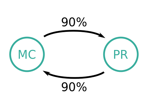
Fig. 6.1 There is a one to one connection between a MCTrackCand and a track from the track finder. The MCTrackCand is labeled found and the other track is labeled matched.¶

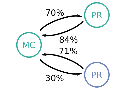
Fig. 6.2 The MCTrackCand is found twice. The track from the track finder with the higher percentage (the green one in this example) is labeled matched, the other one cloned. The MCTrackCand is nevertheless labeled found.¶

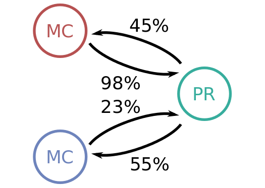
Fig. 6.3 The track from the track finder is created with hits from many different MCTrackCands. As none of the corresponding hit ratios exceeds 66%, the track is called ghost or fake. The hit ratios of the MCTrackCands itself do not play any role here.¶

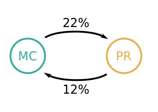
Fig. 6.4 The found track does not describe any of the MCTrackCands well (or well enough) - but is made out of background hits. This track is also called a fake or background.¶

Figures of Merit¶

The four main figures of merit, as also shown on the validation side, are:

Finding efficiency: Number of MC track candidates which are labeled found divided by the total number of MC track candidates
Hit efficiency: Mean of all single hit efficiency of the MC track candidates labeled as found. The single hit efficiency is defined as the number of found hits divided by the number of all hits in a track. This information is encoded in the weight of the relations created by the MCRecoTracksMatcherModule.
Clone rate: Number of PR track candidates which are labeled clone divided by the number of PR track candidates which are labeled clone or matched
Fake rate: Number of PC track candidates which are labeled fake divided by the total number of PR track candidates.

These definitions can be looked up in /tracking/scripts/validation/mc_side_module.py and /tracking/scripts/validation/pr_side_module.py.

6.6.7. Photon matching¶

Details of photon matching efficiency can be found in this talk. If you want to contribute, please feel free to move material from the talk to this section (BII-5316).

6.6.8. Topology analysis¶

This section provides some information on the interface, repositories, and documents of TopoAna, which is a generic tool for the event type analysis of inclusive MC samples in high energy physics experiments, and hence a powerful tool for analysts to investigate the signals and backgrounds involved in their works. TopoAna is an offline tool independent of basf2. It can take the output root files of the Analysis module as input. The MC truth information for the event type analysis can be stored in the root files with the utility MCGenTopo in basf2. Thus, MCGenTopo is the interface of basf2 to TopoAna.

Note

Apart from the interface, this section only introduces the TopoAna resources outside the Belle 2 Software Documentation. Inside the documentation, please see Section 21.5.5 for the online textbook on TopoAna. It is a good idea to start learning the usage of TopoAna with this online textbook. Please feel free to contact Xingyu Zhou (zhouxy@buaa.edu.cn) if you have any questions or comments on TopoAna.

The interface¶

As we mention above, MCGenTopo is the interface of basf2 to TopoAna. To be specific, the interface implements the following parameter function mc_gen_topo(n) in the script variables/MCGenTopo.py.

variables.MCGenTopo.mc_gen_topo(n=200)[source]

Gets the list of variables containing the raw topology information of MC generated events. To be specific, the list including the following variables:

nMCGen: number of MC generated particles in a given event,
MCGenPDG_i (i=0, 1, … n-2, n-1): PDG code of the \({\rm i}^{\rm th}\) MC generated particle in a given event,
MCGenMothIndex_i (i=0, 1, … n-2, n-1): mother index of the \({\rm i}^{\rm th}\) MC generated particle in a given event.

Tip

Internally, nMCGen, MCGenPDG_i and MCGenMothIndex_i are just aliases of nMCParticles, genParticle(i, varForMCGen(PDG)) and genParticle(i, varForMCGen(mcMother(mdstIndex))), respectively.
For more details on the variables, please refer to the documentations of nMCParticles, genParticle, varForMCGen, PDG, mcMother, and mdstIndex.

Parameters: n (int) – number of MCGenPDG_i/MCGenMothIndex_i variables. Its default value is 200.

Note

To completely examine the topology information of the events in an MC sample, the parameter n should be greater than or equal to the maximum of nMCGen in the sample.
Normally, the maximum of nMCGen in the MC samples at Belle II is less than 200. Hence, if you have no idea about the maximum of nMCGen in your own MC sample, it is usually a safe choice to use the default parameter value 200.
However, an overlarge parameter value leads to unncessary waste of disk space and redundant variables with inelegant nan values. Hence, if you know the maximum of nMCGen in your own MC sample, it is a better choice to assign the parameter a proper value.

Below are the steps to use mc_gen_topo(n) to get the input data to TopoAna.

Append the following statement at the beginning part of your python steering script
from variables.MCGenTopo import mc_gen_topo
Use the parameter function mc_gen_topo(n) as a list of variables in the steering function variablesToNtuple as follow
variablesToNtuple(particleList, yourOwnVariableList + mc_gen_topo(n), treeName, fieName, path)
Run your python steering script with basf2

Repositories¶

The following three remote repositories of TopoAna are provided at present. The one at Stash is most convenient to Belle II users. Nonetheless, the two at GitHub and at GitLab of IHEP are also provided as helpful alternatives for possible convenience.

Documents¶

Use cases at Belle II¶

At the end of this section, we list two use cases of TopoAna at Belle II: one for semitauonic analyses and the other for charm analyses. You can refer to them if you work in the related analysis groups.

Using TopoAna with the semitauonic framework by Hannah Marie Wakeling
TopoAna Wrapper for Charm Analysis by Guanda Gong