21.4.9. Continuum Suppression (CS)¶

Introduction¶

Most e⁺ e^- interactions at Belle II do not result in a ϒ(4S) resonance which then decays to two B mesons.

Of these non-ϒ(4S) events, those resulting in some state without hadrons are usually not problematic in analyses looking for B decays as they are already rejected by the trigger.

Continuum events are more problematic. B meson candidates reconstructed from these decays show a broad distribution in variables such as the beam-constrained mass which makes them difficult to separate and suppress when extracting a signal component.

Question

Do you still remember what continuum is?

Hint

Have a look back in Backgrounds, backgrounds, backgrounds where this is introduced.

Solution

When we talk about continuum, we mean events with the process e⁺ e^- → qq, i.e. directly to some lighter hadrons without creating a ϒ(4S) resonance.

In Belle II Monte Carlo, the centrally produced continuum samples are separated by their quark content and are called ‘uubar’, ‘ddbar’, ‘ssbar’ and ‘ccbar’.

If variables which you already know from the previous exercises are bad at separating continuum and BB events, which other properties of the events can we use? The answer is the overall shape of the events, i.e. the momentum-weighted distribution of all particles in the detector.

Question

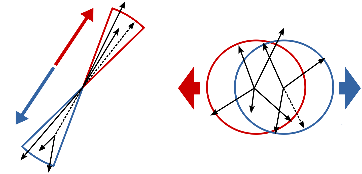
Which of these two pictures better represents the distribution (shape) of particles you would expect in a BB event? Which represents a continuum event?

../../_images/continuum_without_labels.png

Hint

Think about the different masses of the Continuum hadrons compared to B mesons. How does this reflect in the momentum?

Solution

The continuum particles are strongly collimated due to the large available momentum for the decay to light hadrons. In contrast, the particles from the BB event are uniformly distributed.

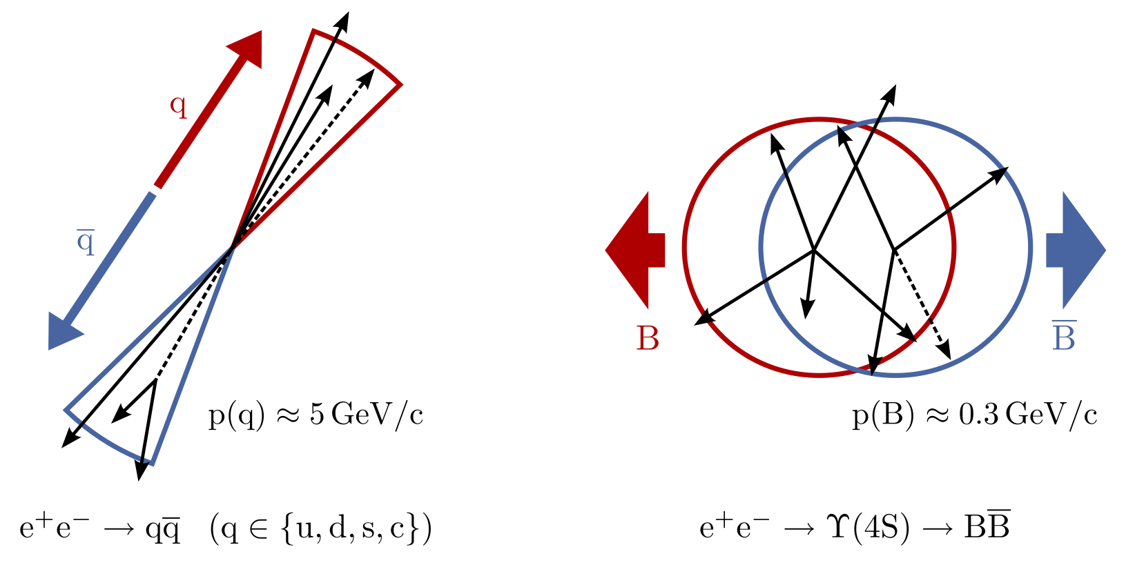
Fig. 21.27 (Credit: Markus Röhrken)¶

So how do we get access to the event shape? We construct B candidates and then create a Rest of Event for them. This allows us to study the entire event and compute shape properties, while taking into account which particles belong to our signal reconstruction.

Warning

In addition to the Continuum Suppression Module module we will be using in this exercise, there is also the Event Shape Framework in basf2 which calculates similar properties to the Continuum Suppression module. However, this does not use candidate-based analysis and is not designed for Continuum Suppression.

Always make sure the variables you’re using in the exercise are from the Continuum Suppression module and not the similarly-named ones from the Event Shape Framework.

Which properties can we use? A popular one is the ratio of the second and zeroth Fox-Wolfram moment:

\[R_2 = \frac{H_2}{H_0}\]

This variable is called R2 in basf2 (not to be confused with foxWolframR2 which is the same property but from the Event Shape Framework).

Fox-Wolfram moments are rotationally-invariant parametrisations of the distribution of particles in an event. They are defined by

\[H_l = \sum_{i,j} \frac{\lvert p_i \rvert \lvert p_j \rvert }{E^2_{\text{event}}} P_l(\cos{\theta_{i, j}})\]

with the momenta p _i,j, the angle θ _i,j between them, the total energy in the event E _event and the Legendre Polynomials P _l.

Other powerful properties are those based on the thrust vector. This is the vector along which the total projection of a collection of momenta is maximised. This collection of momenta can be the B candidate or the rest of event.

The cosine of the angle between both thrust vectors, cosTBTO in basf2, is a thrust-based discriminating variable. In BB events, the particles are almost at rest and so the thrust vectors are uniformly distributed. Therefore, cosTBTO will also be uniformly distributed between 0 and 1. In qq events, the particles are collimated and the thrust axes point back-to-back, leading to a peak at high values of cosTBTO. A similar argument can be made for the angle of the thrust axis with the beam axis which is cosTBz in basf2.

In addition to the angular quantities, basf2 also provides the total thrust magnitude of both the B candidate thrustBm and the ROE thrustOm. Depending on the signal process, these can also provide some discriminating power.

If you would like to know more, Chapter 9 of The Physics of the B Factories book has an extensive overview over these quantities.

Question

Can you find out which other variables are provided by basf2 for continuum suppression?

Hint

Check the Continuum Suppression variable group in Variables.

Solution

In addition to the five variables

mentioned above, basf2 also provides “CLEO cones” (CleoConeCS) and “Kakuno-Super-Fox-Wolfram” variables (KSFWVariables). These are more complex engineered variables and are mostly used with machine learning methods.

First Continuum Suppression steps in basf2¶

Now, how do we access the shape of events in basf2?

First we need some data. In this exercise we will use two samples, one with “uubar” continuum background and one with B → K _S ⁰ 𝜋 ⁰ decays. These samples are called uubar_sample.root and B02ks0pi0_sample.root and can be used with the basf2.find_file function (you need the data_type='examples' switch and also have to prepend starterkit/2021/ to the filename). If this doesn’t work you can find the files in /sw/belle2/examples-data/starterkit/2021 on KEKCC.

Exercise

Load the mdst files mentioned above, then reconstruct Kshort candidates from two charged pions. Load the charged pions with the cut 'chiProb > 0.001 and pionID > 0.5' and combine only pions whose combined invariant mass is within 36 MeV of the neutral kaon mass (498 MeV). We won’t be using the Kshorts from the stdV0s package as these are always vertex fit which we don’t need.

Then, load some neutral pion candidates from stdPi0s and combine them with the Kshort candidates to B0 candidates. Only create B0 candidates with Mbc between 5.1 GeV and 5.3 GeV and deltaE between -2 GeV and 2 GeV.

These cuts are quite loose but this way you will be able to reconstruct B0 candidates from continuum events without processing large amounts of continuum Monte Carlo.

Solution

#!/usr/bin/env python3
import basf2 as b2
import modularAnalysis as ma
import stdPi0s

# Perform analysis.
main = b2.create_path()

ma.inputMdstList(
    environmentType="default",
    filelist=[
        b2.find_file("starterkit/2021/B02ks0pi0_sample.root",
                     data_type="examples"),
        b2.find_file("starterkit/2021/uubar_sample.root",
                     data_type="examples"),
    ],
    path=main,
)

stdPi0s.stdPi0s(path=main, listtype="eff60_Jan2020")
ma.fillParticleList(
    decayString="pi+:good", cut="chiProb > 0.001 and pionID > 0.5", path=main
)

ma.reconstructDecay(
    decayString="K_S0 -> pi+:good pi-:good", cut="0.480<=M<=0.516", path=main
)

ma.reconstructDecay(
    decayString="B0  -> K_S0 pi0:eff60_Jan2020",
    cut="5.1 < Mbc < 5.3 and abs(deltaE) < 2",
    path=main,
)

Exercise

Now, create a Rest of Event for the B0 candidates and append a mask with the track cuts 'nCDCHits > 0 and useCMSFrame(p)<=3.2' and the cluster cuts 'p >= 0.05 and useCMSFrame(p)<=3.2' to it. These cuts are common choices for continuum suppression, however they might not be the best ones for your analysis later on!

Then, adding the continuum suppression module is just a single call to the modularAnalysis.buildContinuumSuppression function. You have to pass the name of the ROE mask you’ve just created to the function.

Hint

You can use modularAnalysis.appendROEMasks to add the mask.

Solution

ma.buildRestOfEvent(target_list_name="B0", path=main)
cleanMask = (
    "cleanMask",
    "nCDCHits > 0 and useCMSFrame(p)<=3.2",
    "p >= 0.05 and useCMSFrame(p)<=3.2",
)
ma.appendROEMasks(list_name="B0", mask_tuples=[cleanMask], path=main)

ma.buildContinuumSuppression(list_name="B0", roe_mask="cleanMask", path=main)

Exercise

Now you can write out a few event shape properties. Use the five properties mentioned above. To evaluate the performance of these variables, add the truth-variable isContinuumEvent.

You can also add the beam-constrained mass Mbc which you should know from previous exercises to see the uniform background component in this variable.

Then, process the path and run the steering file!

Solution

simpleCSVariables = [
    "R2",
    "thrustBm",
    "thrustOm",
    "cosTBTO",
    "cosTBz",
]

ma.variablesToNtuple(
    decayString="B0",
    variables=simpleCSVariables + ["Mbc", "isContinuumEvent"],
    filename="ContinuumSuppression.root",
    treename="tree",
    path=main,
)

b2.process(main)

Now that we have created our ntuple, we can look at the data and see how well the variables suppress continuum.

Exercise

Plot the distributions of R2 from 0 to 1 for both continuum and signal components as determined by isContinuumEvent.

Where would you put the cut when trying to retain as much signal as possible?

If you want you can also plot the other four variables and see how their performance compares.

Hint

Use histtype='step' when plotting with matplotlib, this makes it easier to see the difference between the two distributions.

Solution

# Include this only if running in a Jupyter notebook
%matplotlib inline

import matplotlib.pyplot as plt
from root_pandas import read_root

df = read_root('ContinuumSuppression.root')

fig, ax = plt.subplots()

signal_df = df.query('(isContinuumEvent == 0.0)')
continuum_df = df.query('(isContinuumEvent == 1.0)')

n, bins, patches = ax.hist(signal_df['R2'], bins=30, range=(0, 1), label='Not Continuum', histtype='step')
n, bins, patches = ax.hist(continuum_df['R2'], bins=30, range=(0, 1), label='Continuum', histtype='step')
ax.set_xlabel('R2')
ax.set_ylabel('Total number of candidates')
ax.legend()
fig.savefig('R2.pdf')

Your plot should look similar to this:

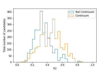
Judging by this plot, a cut at R2 = 0.4 would provide good separation. Of course, this can change if you employ cuts on other CS variables too!

Exercise

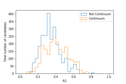
In the previous exercise we have used a uubar sample as our continuum sample. How would you expect the distribution in R2 to change when we switch this out with a ccbar sample? Think about this for a bit, then try it! You can use the file ccbar_sample.root in the starterkit folder.

Solution

The separation becomes worse as the charmed hadrons are heavier and have less momentum:

So how do we separate our signal component from continuum background in the presence of all types of continuum? As you have seen with the five variables we have introduced so far, none of them can provide perfect separation. Fortunately, there is a solution to this: Boosted Decision Trees!

[To be continued…]

Stuck? We can help!

If you get stuck or have any questions to the online book material, the #starterkit-workshop channel in our chat is full of nice people who will provide fast help.

Refer to Collaborative Tools. for other places to get help if you have specific or detailed questions about your own analysis.

Improving things!

If you know how to do it, we recommend you to report bugs and other requests with JIRA. Make sure to use the documentation-training component of the Belle II Software project.

If you just want to give very quick feedback, use the last box “Quick feedback”.

Please make sure to be as precise as possible to make it easier for us to fix things! So for example:

typos (where?)
missing bits of information (what?)
bugs (what did you do? what goes wrong?)
too hard exercises (which one?)
etc.

If you are familiar with git and want to create your first pull request for the software, take a look at How to contribute. We’d be happy to have you on the team!

Quick feedback!

Authors of this lesson

Moritz Bauer