First steering file

3.4.2. First steering file#

In this hands-on tutorial you’ll be writing your first steering file. Our ultimate goal is to reconstruct $B^0 \to J/\Psi(\to e^+e^-)K_S^0(\to \pi^+\pi^+)$. You’ll be learning step-by-step what is necessary to achieve this, and in the end you will produce a plot of the $B$ meson candidates. As you have already learned in the previous sections, basf2 provides a large variety of functionality. While the final steering file of this lesson will be working and producing some reasonable output, there are many possible extensions that you will learn all about in the succeeding lessons.

Let’s get started: The very first step is always to set up the necessary environment.

Task

Set up the basf2 environment using the currently recommended software version.

Hint

Go back to The basics. to see the step-by-step instructions.

Solution

source /cvmfs/belle.cern.ch/tools/b2setup
b2help-releases
b2setup <release-shown-at-prompt-by-previous-script>

Now let’s get started with your steering file!

Task

Open an empty file with an editor of your choice. Add three lines that do the following:

Import the basf2 python library (it might be convenient to set an abbreviation, e.g. b2)
Create a basf2.Path (call it main)
Process the path with basf2.process

Save the file as myanalysis.py.

Hint

Have a look at basf2 and basf2.process

Solution

import basf2 as b2
main = b2.Path()
b2.process(main)

Running steering files is as easy as calling basf2 myanalysis.py on the command-line.

Exercise

Run the short script that you just created. Don’t worry, if you’ve done everything correct, you should see some error messages. Read them carefully!

Solution

The output should look like this:

[INFO] Steering file: myanalysis.py
[INFO] Starting event processing, random seed is set to '94887e3828c78b3bd0b761678bd255317f110e183c2ed59ebdcd027e7610b9d6'
[ERROR] There is no module that provides event and run numbers (EventMetaData). You must add either the EventInfoSetter or an input module (e.g. RootInput) to the beginning of your path.
[FATAL] 1 ERROR(S) occurred! The processing of events will not be started.  { function: void Belle2::EventProcessor::process(const PathPtr&, long int) }
[INFO] ===Error Summary================================================================
[FATAL] 1 ERROR(S) occurred! The processing of events will not be started.
[ERROR] There is no module that provides event and run numbers (EventMetaData). You must add either the EventInfoSetter or an input module (e.g. RootInput) to the beginning of your path.
[INFO] ================================================================================
[ERROR] in total, 1 errors occurred during processing

The random seed will of course differ in your case.

Loading input data#

Of course, no events could be processed so far because no data has been loaded yet. Let’s do it. As already described in the previous lesson almost all convenience functions that are needed can be found in modularAnalysis.

It is recommended to use inputMdstList or inputMdst. If you look at the source code, you’ll notice that the latter actually calls the more general former.

Exercise

How many arguments are required for the inputMdstList function? Which value has to be set for the environment type?

Hint

Take a look at the signature of the function. It is highlighted in blue at the top. Some arguments take a default value, e.g. skipNEvents=0 and are therefore not required.

Solution

Two parameters have no default value and are therefore required:

a list of root input files
the path

The environmentType only has to be modified if you are analyzing Belle data / MC.

In a later lesson you’ll learn how and where to find input files for your analysis. For the purpose of this tutorial we have prepared some local input files of $B^0 \to J/\Psi K_S^0$. They should be available in the ${BELLE2_EXAMPLES_DATA_DIR}/starterkit/2021 directory on KEKCC, NAF, and other servers. The files’ names start with the decfile number 1111540100.

If you’re working from an institute server

Perhaps you are working on the server of your home institute and this folder is not available. In this case please talk to your administrators to make the ${BELLE2_EXAMPLES_DATA_DIR} available for you and make sure that it is synchronized. Note that we might not be able to provide you with the same level of support on other machines though.

If you’re working on your own machine

In this case you might first need to copy the data files to your home directory on your local machine from kekcc or DESY via an SSH connection (cf. SSH - Secure Shell) and then either change the path accordingly or set the BELLE2_EXAMPLES_DATA_DIR environment variable to point to the right directory. Note that we might not be able to provide you with the same level of support on other machines though.

Exercise

Check out the location of the files mentioned above. Which two settings of MC are provided?

Hint

Remember the ls (and cd) bash command?

Solution

ls ${BELLE2_EXAMPLES_DATA_DIR}/starterkit/2021

Alternatively, you can first navigate to the directory with cd and then just call ls without any arguments.

There are each 10 files with and without beam background (BGx1 and BGx0). Their names only differ by the final suffix, which is an integer between 0 and 9.

A helpful function to get common data files from the examples directory is basf2.find_file.

Task

Extend your steering file by loading the data of one of the local input files. It makes sense to run the steering file again.

If there is a syntax error in your script or you forgot to include a necessary argument, there will be an error message that should help you to debug and figure out what needs to be fixed.
If the script is fine, only three lines with info messages should be printed to the output and you should see a quickly finishing progress bar.

Hint

Don’t forget to import modularAnalysis (this is the module that contains inputMdstList). It might be convenient to set an abbreviation, e.g. ma. Then you have to set the correct values for the two required arguments of inputMdstList.

Solution

#!/usr/bin/env python3

import basf2 as b2
import modularAnalysis as ma

# create path
main = b2.Path()

# load input data from mdst/udst file
ma.inputMdstList(
    filelist=[b2.find_file("starterkit/2021/1111540100_eph3_BGx0_0.root", "examples")],
    path=main
)

# start the event loop (actually start processing things)
b2.process(main)

In the solution to the last task we have added empty lines, some comments, and used shortcuts for the imports. This helps to give the script a better structure and allows yourself and others to better understand what’s going on in the steering file. In the very first line we have also added a shebang to define that the steering file should be executed with a python interpreter.

So far, the input file has been completely hard-coded. But as we’ve seen before the file names only differ by the final suffix. We can add a little bit more flexibility by providing this integer as a command-line argument. Then, we can select a different input file when running the steering file without having to change anything in the script itself.

Task

Adjust your steering file so that you can select via an integer as a command-line argument which file is going to be processed.

Hint

You should have learned about command-line arguments in this part of the python introduction from Software Carpentry. Otherwise, go back and refresh your memory. All you have to do is to import the system library, store the correct command-line argument (from sys.argv) in a local variable filenumber, and extend the path string to include it.

Hint

You can get the integer from the command line arguments using

import sys

filenumber = sys.argv[1]

Hint

Rather than concatenating strings with + ("file_" + str(filenumber) + ".root"), you can also use so-called f-strings: f"file_{filenumber}.root". They are great for both readability and performance.

Solution

#!/usr/bin/env python3

import sys
import basf2 as b2
import modularAnalysis as ma

# get input file number from the command line
filenumber = sys.argv[1]

# create path
main = b2.Path()

# load input data from mdst/udst file
ma.inputMdstList(
    filelist=[b2.find_file(f"starterkit/2021/1111540100_eph3_BGx0_{filenumber}.root", "examples")],
    path=main,
)

# start the event loop (actually start processing things)
b2.process(main)

Tip

Make sure that from now on you always supply a number every time you run your steering file, e.g. basf2 myanalysis.py 1.

Otherwise you will get an exception like this

Traceback (most recent call last):
  File "myanalysis.py", line 3, in <module>
    filenumber = sys.argv[1]
IndexError: list index out of range

Filling particle lists#

The mdst data objects (Tracks, ECLCluster, KLMCluster, V0s) of the input file have to be transferred into Particle data objects. This is done via the ParticleLoader module and its wrapper function (convenience function) fillParticleList.

Exercise

Read the documentation of fillParticleList to familiarize yourself with the required arguments.

Which six final state particles can be created from Tracks?

Solution

Electrons, muons, pions, kaons, protons, and deuterons.

Internally, the anti-particle lists are always filled as well, so it is not necessary to call fillParticleList for e+ and e-. In fact, you will see a warning message for the second call telling you that the corresponding particle list already exists.

As long as no selection criteria (cuts) are provided, the only difference between loading different charged final state particle types is the mass hypothesis used in the track fit.

Each particle used in the decayString argument of the fillParticleList function can be extended with a label. This is useful to distinguish between multiple lists of the same particle type with different selection criteria, e.g. soft and hard electrons.

ma.fillParticleList("e-:soft", "E < 1", path=main) # the label of this electron list is "soft"
ma.fillParticleList("e-:hard", "E > 3", path=main) # here the label is "hard"

Warning

If the provided cut string is not empty you can not use the label all, i.e. having

ma.fillParticleList("e-:all", "E > 0", path=main)

in your steering file will cause a fatal error and stop the execution of your script.

There are standard particle lists with predefined selection criteria. While those for charged final state particles should only be used in the early stages of your analysis and be replaced with dedicated selections adjusted to the needs of the decay mode you are studying, it is recommended to use them for V0s ($K_S^0$, $\Lambda^0$). They are part of the library stdV0s.

Exercise

Find the documentation of the convenience function that creates the standard $K_S^0$ particle list. What is the name of the particle list generated by this function?

Hint

The documentation is here: stdV0s.stdKshorts.

Solution

It’s K_S0:merged because it is a combination of $K_S^0$ candidates created directly from V0s found in the tracking and combinations of two charged pions.

Task

Extend your steering file by loading electrons, positrons, and $K_S^0$ candidates.

Hint

All you need is fillParticleList and stdKshorts. Remember that charge-conjugated particles are automatically created. You do not need a cut for the electrons, so you can use an empty string "".

Hint

Always keep in mind from which module your functions are taken. Since stdKshorts comes from the module stdV0s, you need to import it first.

Solution

#!/usr/bin/env python3

import sys
import basf2 as b2
import modularAnalysis as ma
import stdV0s

# get input file number from the command line
filenumber = sys.argv[1]

# create path
main = b2.Path()

# load input data from mdst/udst file
ma.inputMdstList(
    filelist=[b2.find_file(f"starterkit/2021/1111540100_eph3_BGx0_{filenumber}.root", "examples")],
    path=main,
)

# fill final state particle lists
ma.fillParticleList("e+:uncorrected", "", path=main)
stdV0s.stdKshorts(path=main)

# Start the event loop (actually start processing things)
b2.process(main)

In the solution we gave the electrons the label uncorrected. This is already in anticipation of a future extension in which Bremsstrahlung recovery will be applied (Various additions).

Task

Run your steering file and answer the following questions:

Which are the mass window boundaries set for the $K_S^0$?

Hint

Don’t forget to include a number, e.g. 1 as a command line argument to specify the input file number!

Solution

basf2 myanalysis.py 1

In the output there are INFO messages that the $K_S^0$ invariant mass has to be between 0.45 and 0.55 GeV/c ².

In the previous task you should have learned how useful it is to carefully study the output. This is especially relevant if there are warning or error messages. Remember to never ignore them as they usually point to some serious issue, either in the way you have written your steering file or in the basf2 software itself. In the latter case you are encouraged to report the problem so that it can be fixed by some experts (maybe you yourself will become this expert one day).

In order to purify a sample it makes sense to apply at least loose selection criteria. This can be based on the particle identification (e.g. electronID for electrons and positrons), requiring the tracks to originate from close to the interaction point (by using dr and dz), and having a polar angle in the acceptance of the CDC (thetaInCDCAcceptance).

Exercise

Find out what’s the difference between dr and dz, e.g. why do we not have to explicitly ask for the absolute value of dr? What’s the angular range of the CDC acceptance (as implemented in the software)?

Hint

The documentation of dr and dz should tell you all about the first question. The angular range is a bit trickier. You have to directly inspect the source code of the variable defined in the variables folder of the analysis package. There has been an exercise on how to find the source code in Getting started, and getting help interactively.

Solution

The variable dr gives the transverse distance, while dz is the z-component of the point of closest approach (POCA) with respect to the interaction point (IP). Components are signed, while distances are magnitudes.

The polar range of the CDC acceptance is $17^\circ < \theta < 150^\circ$ as written here.

Task

Apply a cut on the electron particle list, requiring an electron ID greater than 0.1, a maximal transverse distance to the IP of 0.5 cm, a maximal distance in z-direction to the IP of 2 cm, and the track to be inside the CDC acceptance.

Hint

Previously we were using an empty string "" as argument to fillParticleList. Now you need to change this.

Solution

ma.fillParticleList(  # [S10]
    "e+:uncorrected",
    "electronID > 0.1 and dr < 0.5 and abs(dz) < 2 and thetaInCDCAcceptance",
    path=main,
)  # [E10]

Note

Marker comments in the solution code

If you are wondering about comments like [S10] or [E10] in the code snippets that we include in our tutorials: You can completely ignore them. In case you are curious about their meaning: Sometimes we want to show only a small part of a larger file. Copying the code or referencing the lines by line numbers is a bit unstable (what if someone changes the code and forgets to update the rest of the documentation?), so we use these tags to mark the beginning and end of a subset of lines to be included in the documentation.

Combining particles#

Now we have a steering file in which final state particles are loaded from the input mdst file to particle lists. One of the most powerful modules of the analysis software is the ParticleCombiner. It takes those particle lists and finds all unique combinations. The same particle can of course not be used twice, e.g. the two positive pions in $D^0 \to K^- \pi^+ \pi^+ \pi^-$ have to be different mdst track objects. However, all of this is taken care of internally. For multi-body decays like the one described above, there can easily be many multiple candidates which share some particles but differ by at least one final state particle.

The wrapper function for the ParticleCombiner is called reconstructDecay. Its first argument is a DecayString, which is a combination of a mother particle (list), an arrow, and daughter particles. The DecayString has its own grammar with several markers, keywords, and arrow types. It is especially useful for inclusive reconstructions (reconstructions in which only part of the decay products are specified, e.g. only requiring charged leptons in the final state; the opposite would be exclusive reconstructions). Follow the provided link if you want to learn more about the DecayString. For the purpose of this tutorial, we do not need any of those fancy extensions as the default arrow type -> suffices. However, it is important to know how the particles themselves need to be written in the decay string.

Exercise

How do we have to type a $J/\Psi$, and what is its nominal mass?

Hint

Make use of the tool b2help-particles (basf2 particles). As a spin-1 $c\bar{c}$ resonance the PDG code of the $J/\Psi$ is 443.

Solution

The $J/\Psi$ has to be typed J/psi. Whenever you misspell a particle name in a decay string, there will be an error message telling you that it is unknown.

The invariant mass of the $J/\Psi$ is set to 3.0969 GeV/c ².

Task

Extend the steering file by first forming $J/\Psi$ candidates from electron-positron combinations, and then combining them with a $K_S^0$ to form $B^0$ candidates.

Include a abs(dM) < 0.11 cut for the $J/\Psi$.

Hint

All you need is to call reconstructDecay twice.

Hint

The $J/\Psi$ reconstruction looks like this:

# combine final state particles to form composite particles [S20]
ma.reconstructDecay(
    "J/psi:ee -> e+:uncorrected e-:uncorrected", cut="abs(dM) < 0.11", path=main
)  # [E20]

Solution

#!/usr/bin/env python3

import sys
import basf2 as b2
import modularAnalysis as ma
import stdV0s

# get input file number from the command line
filenumber = sys.argv[1]

# create path
main = b2.Path()

# load input data from mdst/udst file
ma.inputMdstList(
    filelist=[b2.find_file(f"starterkit/2021/1111540100_eph3_BGx0_{filenumber}.root", "examples")],
    path=main,
)

# fill final state particle lists
ma.fillParticleList(  # [S10]
    "e+:uncorrected",
    "electronID > 0.1 and dr < 0.5 and abs(dz) < 2 and thetaInCDCAcceptance",
    path=main,
)  # [E10]
stdV0s.stdKshorts(path=main)

# combine final state particles to form composite particles [S20]
ma.reconstructDecay(
    "J/psi:ee -> e+:uncorrected e-:uncorrected", cut="abs(dM) < 0.11", path=main
)  # [E20]

# combine J/psi and KS candidates to form B0 candidates
ma.reconstructDecay(
    "B0 -> J/psi:ee K_S0:merged",
    cut="",
    path=main,
)
#  [E30]

Writing out information to an ntuple#

To separate signal from background events, and to extract physics parameters, an offline analysis has to be performed. The final step of the steering file is to write out information in a so called ntuple using variablesToNtuple. It can contain one entry per candidate or one entry per event.

Exercise

How do you switch between the two ntuple modes?

Hint

Look at the documentation of variablesToNtuple.

Solution

When providing an empty decay string, an event-wise ntuple will be created.

Warning

Only variables declared as Eventbased are allowed in the event mode. Conversely, both candidate and event-based variables are allowed in the candidate mode.

A good variable to start with is the beam-constrained mass Mbc, which is defined as

\[\text{M}_{\rm bc} = \sqrt{E_{\rm beam}^2 - \mathbf{p}_{B}^2}\]

For correctly reconstructed $B$ mesons this variable should peak at the $B$ meson mass.

Task

Add some code that saves the beam-constrained $B$ mass of each $B$ candidate in an output ntuple. Then, run your steering file.

Hint

The variable for the beam-constrained $B$ mass is called Mbc. It has to be provided as an element of a list to the argument variables of the variablesToNtuple function.

Solution

#!/usr/bin/env python3

import sys
import basf2 as b2
import modularAnalysis as ma
import stdV0s

# get input file number from the command line
filenumber = sys.argv[1]

# create path
main = b2.Path()

# load input data from mdst/udst file
ma.inputMdstList(
    filelist=[b2.find_file(f"starterkit/2021/1111540100_eph3_BGx0_{filenumber}.root", "examples")],
    path=main,
)

# fill final state particle lists
ma.fillParticleList(  # [S10]
    "e+:uncorrected",
    "electronID > 0.1 and dr < 0.5 and abs(dz) < 2 and thetaInCDCAcceptance",
    path=main,
)  # [E10]
stdV0s.stdKshorts(path=main)

# combine final state particles to form composite particles [S20]
ma.reconstructDecay(
    "J/psi:ee -> e+:uncorrected e-:uncorrected", cut="abs(dM) < 0.11", path=main
)  # [E20]

# combine J/psi and KS candidates to form B0 candidates
ma.reconstructDecay(
    "B0 -> J/psi:ee K_S0:merged",
    cut="",
    path=main,
)
#  [E30]
# save variables to an output file (ntuple)
ma.variablesToNtuple(
    "B0",
    variables=['Mbc'],
    filename="Bd2JpsiKS.root",
    treename="tree",
    path=main,
)

# start the event loop (actually start processing things)
b2.process(main)

Although you are analyzing a signal MC sample, the reconstruction will find many candidates that are actually not signal, but random combinations that happen to fulfill all your selection criteria.

Task

Write a short python script in which you load the root ntuple from the previous exercise into a dataframe and then plot the distribution of the beam-constrained mass using a histogram with 100 bins between the range 4.3 to 5.3 GeV/c ².

Can you identify the signal and background components?

Hint

Read in the ntuple using uproot. Use the histogram plotting routine of the dataframe. For instructions on the basic usage of uproot see the Getting started guide.

Hint

You might take a look back at your python training. This is a good use case for a jupyter notebook. Make sure to include the %matplotlib inline magic to see the plots.

Solution

import matplotlib.pyplot as plt
import uproot

df = uproot.open('Bd2JpsiKS.root:tree').arrays(['Mbc'], library='pd')

df.hist('Mbc', bins=100, range=(4.3, 5.3))
plt.xlabel(r'M$_{\rm bc}$ [GeV/c$^{2}$]')
plt.ylabel('Number of candidates')
plt.xlim(4.3, 5.3)
plt.savefig('Mbc_all.png')

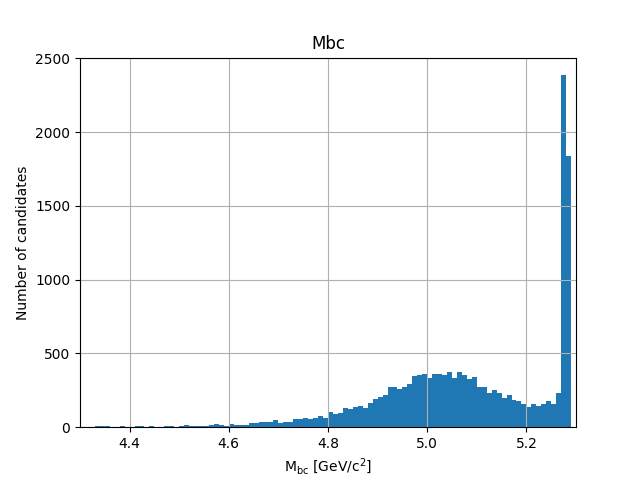
../../_images/Mbc_all.png — Fig. 3.21 There is a (signal) peak at the nominal $B$ mass of 5.28 GeV/c ² and lots of background candidates as a broad bump left of the peak.#

Adding MC information#

For the beam-constrained mass we know pretty well how the signal distribution should look like. But what’s the resolution and how much background actually extends under the signal peak? With MC, we have the advantage that we know what has been generated. Therefore, we can add a flag to every candidate to classify it as signal or background. Furthermore, we can study our background sources if we know what the reconstruction has falsely identified.

There is a long chapter on MC matching in the documentation. You should definitely read it to understand at least the basics.

Exercise

Which module do you have to run to get the relations between the reconstructed and the generated particles? How often do you have to call the corresponding function?

Hint

Did you have a look at the documentation of MC matching?

Solution

You need to run the MCMatcherParticles module, most conveniently available via the wrapper function modularAnalysis.matchMCTruth. If this is run on the head of the decay chain, it only needs to be called once because the relations of all (grand)^N-daughter particles are set recursively.

Task

Add MC matching for all particles of the decay chain, and save information on whether the reconstructed $B$ meson is a signal candidate to the ntuple. Run the steering file again.

Hint

Only one line of code is needed to call matchMCTruth.

Hint

Which variable is added by matchMCTruth? Remember to add it to the ntuple!

Solution

#!/usr/bin/env python3

import sys
import basf2 as b2
import modularAnalysis as ma
import stdV0s

# get input file number from the command line
filenumber = sys.argv[1]

# create path
main = b2.Path()

# load input data from mdst/udst file
ma.inputMdstList(
    filelist=[b2.find_file(f"starterkit/2021/1111540100_eph3_BGx0_{filenumber}.root", "examples")],
    path=main,
)

# fill final state particle lists
ma.fillParticleList(
    "e+:uncorrected",
    "electronID > 0.1 and dr < 0.5 and abs(dz) < 2 and thetaInCDCAcceptance",
    path=main,
)
stdV0s.stdKshorts(path=main)

# combine final state particles to form composite particles
ma.reconstructDecay(
    "J/psi:ee -> e+:uncorrected e-:uncorrected", cut="abs(dM) < 0.11", path=main
)

# combine J/psi and KS candidates to form B0 candidates
ma.reconstructDecay(
    "B0 -> J/psi:ee K_S0:merged",
    cut="",
    path=main,
)

# match reconstructed with MC particles
ma.matchMCTruth("B0", path=main)

# save variables to an output file (ntuple)
ma.variablesToNtuple(
    "B0",
    variables=['Mbc', 'isSignal'],
    filename="Bd2JpsiKS.root",
    treename="tree",
    path=main,
)

# start the event loop (actually start processing things)
b2.process(main)

Task

Plot the beam-constrained mass but this time use the signal flag to visualize which component is signal and which is background.

Hint

Remember the by keyword for df.hist? Alternatively you could also use df.query. The necessary variable is called isSignal.

Solution

import matplotlib.pyplot as plt
import uproot

df = uproot.open('Bd2JpsiKS.root:tree').arrays(['isSignal', 'Mbc'], library='pd')

df.hist('Mbc', bins=100, range=(4.3, 5.3), by='isSignal')
plt.xlabel(r'M$_{\rm bc}$ [GeV/c$^{2}$]')
plt.ylabel('Number of candidates')
plt.xlim(4.3, 5.3)
plt.savefig('Mbc_MCsplit.png')

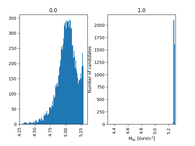
../../_images/Mbc_MCsplit.png — Fig. 3.22 The background peaks around 5 GeV/c ², but does also extend into the signal peak region.#

As you could see, it makes sense to cut on Mbc from below. A complementary variable that can be used to cut away background is $\Delta E$ (deltaE).

Exercise

When combining your $J/\Psi$ with your $K_S^0$, introduce a cut $\text{M}_{\rm bc} > 5.2$ and $|\Delta E|<0.15$.

Hint

Take a look at the cut argument for reconstructDecay. You will also need the abs metafunction.

Solution

# combine J/psi and KS candidates to form B0 candidates [S40]
ma.reconstructDecay(
    "B0 -> J/psi:ee K_S0:merged",
    cut="Mbc > 5.2 and abs(deltaE) < 0.15",
    path=main,
)  # [E40]

Variable collections#

While the MC matching allows us to separate signal from background and study their shapes, we need to use other variables to achieve the same on collision data. Initially, it makes sense to look at many different variables and try to find those with discriminating power between signal and background. The most basic information are the kinematic properties like the energy and the momentum (and its components). In basf2, collections of variables for several topics are pre-prepared. You can find the information in the Collections and Lists section of the documentation.

Exercise

Find out which variable collections contain the variables we have added to the ntuple so far.

Solution

The collection deltae_mbc contains Mbc and deltaE. The isSignal variable along with many other truth match variables is in the collection mc_truth.

Task

Save all the kinematic information, both the truth and the reconstructed values, of the $B$ meson to the ntuple. Also, use the variable collections from the last exercise to replace the individual list.

Hint

The variable collections kinematics, mc_kinematics, deltae_mbc, and mc_truth make your life a lot easier.

Solution

#!/usr/bin/env python3

import sys
import basf2 as b2
import modularAnalysis as ma
import stdV0s
import variables.collections as vc

# get input file number from the command line
filenumber = sys.argv[1]

# create path
main = b2.Path()

# load input data from mdst/udst file
ma.inputMdstList(
    filelist=[b2.find_file(f"starterkit/2021/1111540100_eph3_BGx0_{filenumber}.root", "examples")],
    path=main,
)

# fill final state particle lists
ma.fillParticleList(
    "e+:uncorrected",
    "electronID > 0.1 and dr < 0.5 and abs(dz) < 2 and thetaInCDCAcceptance",
    path=main,
)
stdV0s.stdKshorts(path=main)

# combine final state particles to form composite particles
ma.reconstructDecay(
    "J/psi:ee -> e+:uncorrected e-:uncorrected", cut="abs(dM) < 0.11", path=main
)

# combine J/psi and KS candidates to form B0 candidates [S40]
ma.reconstructDecay(
    "B0 -> J/psi:ee K_S0:merged",
    cut="Mbc > 5.2 and abs(deltaE) < 0.15",
    path=main,
)  # [E40]

# match reconstructed with MC particles
ma.matchMCTruth("B0", path=main)

# Create list of variables to save into the output file
b_vars = []

standard_vars = vc.kinematics + vc.mc_kinematics + vc.mc_truth
b_vars += vc.deltae_mbc
b_vars += standard_vars

# save variables to an output file (ntuple)
ma.variablesToNtuple(
    "B0",
    variables=b_vars,
    filename="Bd2JpsiKS.root",
    treename="tree",
    path=main,
)

# start the event loop (actually start processing things)
b2.process(main)

Hint

If you have trouble understanding what we are doing with the b_vars list, simply add a couple of print(b_vars) between the definition and the operations on it. You might also want to take another look at your understanding of lists.

Variable aliases#

Apart from variables for the mother $B$ meson, we are also interested in the information of the other daughter and granddaughter variables. You can access them via the daughter meta variable, which takes an integer and a variable name as input arguments. The integer (0-based) counts through the daughter particles, e.g. daughter(0, p) would be the momentum of the first daughter, in our case of the $J/\Psi$. This function can also be used recursively.

Exercise

What does daughter(0, daughter(0, E)) denote?

Solution

It’s the energy of the positive electron.

In principle, one can add these nested variables directly to the ntuple, but the brackets have to be escaped (i.e. replaced with “normal” characters), and the resulting variable name in the ntuple is not very user-friendly or intuitive. For example daughter(0, daughter(0, E)) becomes daughter__bo0__cm__spdaughter__bo0__cm__spE__bc__bc. Not exactly pretty, right?

So instead, let’s define aliases to translate the variable names! This can be done with addAlias.

Exercise

How can you replace daughter(0, daughter(0, E)) with ep_E?

Hint

Check the documentation of addAlias for the correct syntax.

Solution

from variables import variables as vm

vm.addAlias("ep_E", "daughter(0, daughter(0, E))")

However, this can quickly fill up many, many lines. Therefore, there are utils to easily create aliases. The most useful is probably create_aliases_for_selected. It lets you select particles from a decay string via the ^ operator for which you want to define aliases, and also set a prefix. Another utility is create_aliases, which is particularly useful to wrap a list of variables in another meta-variable like useCMSFrame or matchedMC.

Task

Add PID and track variables for all charged final state particles and the invariant mass of the intermediate resonances to the ntuple. Also, add the standard variables from before for all particles in the decay chain, and include the kinematics both in the lab and the CMS frame.

Hint: Where to look

You need the variable collections and alias functions mentioned above! Take it one step at a time, it’s more lines of code than in the previous examples.

Hint: Partial solution for final state particles

This is how we add variables to the final state particles:

# variables for final states (electrons, positrons, pions) [S50]
fs_vars = vc.pid + vc.track + vc.track_hits + standard_vars
b_vars += vu.create_aliases_for_selected(
    fs_vars,
    "B0 -> [J/psi -> ^e+ ^e-] [K_S0 -> ^pi+ ^pi-]",
    prefix=["ep", "em", "pip", "pim"],
)  # [E50]

Next, do the same for the $J/\Psi$ and the $K_S^0$ in a similar fashion.

Hint: CMS variables

The bit about the CMS variables is tricky. First create a variable cmskinematics with the create_aliases function. Use “CMS” as the prefix. What do you need to specify for the wrapper? Then use your cmskinematics variable together with create_aliases_for_selected to add these variables to the relevant particles.

Hint: Partial solution for the CMS variables

This is the code for the first part of the last hint:

# also add kinematic variables boosted to the center of mass frame (CMS) [S60]
# for all particles
cmskinematics = vu.create_aliases(
    vc.kinematics, "useCMSFrame({variable})", "CMS"
)  # [E60]

Solution

#!/usr/bin/env python3

import sys
import basf2 as b2
import modularAnalysis as ma
import stdV0s
import variables.collections as vc
import variables.utils as vu

# get input file number from the command line
filenumber = sys.argv[1]

# create path
main = b2.Path()

# load input data from mdst/udst file
ma.inputMdstList(
    filelist=[b2.find_file(f"starterkit/2021/1111540100_eph3_BGx0_{filenumber}.root", "examples")],
    path=main,
)

# fill final state particle lists
ma.fillParticleList(
    "e+:uncorrected",
    "electronID > 0.1 and dr < 0.5 and abs(dz) < 2 and thetaInCDCAcceptance",
    path=main,
)
stdV0s.stdKshorts(path=main)

# combine final state particles to form composite particles
ma.reconstructDecay(
    "J/psi:ee -> e+:uncorrected e-:uncorrected", cut="abs(dM) < 0.11", path=main
)

# combine J/psi and KS candidates to form B0 candidates
ma.reconstructDecay(
    "B0 -> J/psi:ee K_S0:merged",
    cut="Mbc > 5.2 and abs(deltaE) < 0.15",
    path=main,
)

# match reconstructed with MC particles
ma.matchMCTruth("B0", path=main)

# create list of variables to save into the output file
b_vars = []

standard_vars = vc.kinematics + vc.mc_kinematics + vc.mc_truth
b_vars += vc.deltae_mbc
b_vars += standard_vars

# variables for final states (electrons, positrons, pions) [S50]
fs_vars = vc.pid + vc.track + vc.track_hits + standard_vars
b_vars += vu.create_aliases_for_selected(
    fs_vars,
    "B0 -> [J/psi -> ^e+ ^e-] [K_S0 -> ^pi+ ^pi-]",
    prefix=["ep", "em", "pip", "pim"],
)  # [E50]

# variables for J/Psi, KS
jpsi_ks_vars = vc.inv_mass + standard_vars
b_vars += vu.create_aliases_for_selected(jpsi_ks_vars, "B0 -> ^J/psi ^K_S0")

# also add kinematic variables boosted to the center of mass frame (CMS) [S60]
# for all particles
cmskinematics = vu.create_aliases(
    vc.kinematics, "useCMSFrame({variable})", "CMS"
)  # [E60]
b_vars += vu.create_aliases_for_selected(
    cmskinematics, "^B0 -> [^J/psi -> ^e+ ^e-] [^K_S0 -> ^pi+ ^pi-]"
)

# save variables to an output file (ntuple)
ma.variablesToNtuple(
    "B0",
    variables=b_vars,
    filename="Bd2JpsiKS.root",
    treename="tree",
    path=main,
)

# start the event loop (actually start processing things)
b2.process(main)

Hint

To get more information about the aliases we are creating, simply use VariableManager.printAliases (vm.printAliases()) just before processing your path.

First steering file

Contents

3.4.2. First steering file#

Loading input data#

Filling particle lists#

Combining particles#

Writing out information to an ntuple#

Adding MC information#

Variable collections#

Variable aliases#