Various additions

3.4.4. Various additions#

What is Bremsstrahlung radiation?#

As you may guess from its unfriendly typing, “Bremsstrahlung” is a German word, literally meaning “braking radiation”; it is used to describe the electromagnetic radiation that particles emit when decelerating. You can read more about it in the many, many pages available on the Internet, starting with Wikipedia and the PDG review.

At Belle II, Bremsstrahlung radiation is emitted by particles when traversing the different detector components. As the largest material load is near the interaction region, most Bremsstrahlung radiation is expected to originate there. The total radiated power due to Bremsstrahlung by a particle of charge $q$ moving at speed (in units of $c$) $\beta$ is given by

\[P = \frac{q^2\gamma^6}{6\pi\varepsilon_0 c} \left( \left(\dot{\vec{\beta}}\right)^2 - \left(\vec{\beta} \times \dot{\vec{\beta}}\right)^2 \right)\]

where $\gamma = \frac{1}{\sqrt{1-\beta^2}}$.

For cases where the acceleration is parallel to the velocity, the radiated power is proportional to $\gamma^6$, whereas for perpendicular acceleration it scales with $\gamma^4$. As $\gamma = E/mc^2$, lighter particles will lose more energy through Bremsstrahlung than heavier particles with the same energy. At Belle II, we usually only consider Bremsstrahlung loses for electrons and positrons.

Exercise (optional)

From the general equation for radiated power, derive the explicit form for the limit cases of perpendicular and parallel acceleration (if you are attending the Starter Kit, you may want to try this later, so it doesn’t interfere with the flow of the lesson).

Hint

The case of parallel acceleration and velocity should be straightforward. For the perpendicular case, the next identity may be useful:

\[\left(\vec{\beta}\cdot \dot{\vec{\beta}}\right)^2 = \dot{\beta}^2\beta^2 - \left(\vec{\beta} \times \dot{\vec{\beta}}\right)^2\]

Solution

\[P_{a\parallel v} = \frac{q^2a^2\gamma^6}{6\pi\varepsilon_0c^3} \hspace{1cm} P_{a\bot v} = \frac{q^2a^2\gamma^4}{6\pi\varepsilon_0c^3}\]

A proper method that accounts for Bremsstrahlung loses is of utmost importance at B factories; at the end of this section, you will be able to obtain the invariant mass distribution for the $J/\psi \to e^+e^-$ meson decay after correcting for the Bremsstrahlung radiation, and compare it with the distribution you obtained in the previous lesson.

How do we look for Bremsstrahlung photons#

Though we will not discuss it here (but, if you are interested, you can consult this document), the radiated power for relativistic particles is maximum around the particle’s direction of motion; we thus expect Bremsstrahlung photons to be mostly emitted in a cone around the momentum vector of the electrons (and positrons). The procedures we use to perform Bremsstrahlung recovery are based on this assumption.

The Belle like recovery looks for photons on a single cone around the initial momentum of the particle; on the other side, the Belle II method uses multiple cones, centered around the momentum of the particle at the points along its path where it was more likely to emit Bremsstrahlung radiation. The Belle II method also performs a pre-processing of the data, and applies some initial cuts on the Bremsstrahlung photons and on the electrons which the user cannot undo. Although we recommend using the Belle II method, you should check which procedure works best for your analysis.

In order to perform Bremsstrahlung recovery (either with the Belle or the Belle II methods), you need first to construct two particle lists: the first one will have the particles whose energies you want to recover, and the second one will contain the Bremsstrahlung photons you will use to recover said energies. Making use of the steering file developed in the previous sections, we already have our first particle list ready: e+:uncorrected (the reason why this particle list was given this name is, well, because these positrons haven’t been Bremsstrahlung corrected yet!).

Next we will build up the list of possible Bremsstrahlung photons. In order to reduce the number of background clusters included, we first define a minimum cluster energy according to the region in the ECL the cluster is found.

Because this cut will be a bit complicated, we will define aliases for cuts. This actually works with the addAlias function as well, if we combine it with the passesCut function.

Exercise

How would you define the alias myCut for the cut E > 1 and p > 1?

Solution

You can use the passesCut function to turn a cut into a variable and assign an alias for it.

from variables import variables as vm
vm.addAlias("myCut", "passesCut(E > 1 and p > 1")

Exercise

Create a particle list, called gamma:brems, with photons following the next cuts:

If the photons are in the forward endcap of the ECL, their energy should be at least 75 MeV
If they are in the barrel region, their energy should be larger than 50 MeV
Finally, if they are in the backward endcap, their energy should be larger than 100 MeV

To do this, you need the clusterReg and clusterE variable. To keep everything neat and tidy, we recommend that you define the aliases goodFWDGamma, goodBRLGamma and goodBWDGamma for the three cuts. Finally you can combine them to a goodGamma cut and use this to fill the particle list.

Hint

The cuts will look like this:

vm.addAlias(
    "goodXXXGamma", "passesCut(clusterReg == XXX and clusterE > XXX)"
)

where the XXX should be filled by you.

Another hint

This is the first one:

# apply Bremsstrahlung correction to electrons [S10|S20]
vm.addAlias(
    "goodFWDGamma", "passesCut(clusterReg == 1 and clusterE > 0.075)"
)  # [E10]

Solution

# apply Bremsstrahlung correction to electrons [S10|S20]
vm.addAlias(
    "goodFWDGamma", "passesCut(clusterReg == 1 and clusterE > 0.075)"
)  # [E10]
vm.addAlias(
    "goodBRLGamma", "passesCut(clusterReg == 2 and clusterE > 0.05)"
)
vm.addAlias(
    "goodBWDGamma", "passesCut(clusterReg == 3 and clusterE > 0.1)"
)
vm.addAlias(
    "goodGamma", "passesCut(goodFWDGamma or goodBRLGamma or goodBWDGamma)"
)  # [E20]

Next, we perform the actual recovery, using the correctBrems function in the Modular Analysis package.

This step will create a new particle list; each particle in this list will have momentum given by the sum of the original, uncorrected particle momentum, and the momenta of all the Bremsstrahlung photons in the gamma:brems list that fall inside the cone(s) we mentioned previously. Each new particle will also have as daughters the original particle and its Bremsstrahlung photons (if any), and an extraInfo field named bremsCorrected that will indicate if at least one Bremsstrahlung photon was added to this particle.

Exercise

Perform Bremsstrahlung recovery on the e+:uncorrected list, using the correctBrems function and the gamma:brems photons. Create a new variable, called isBremsCorrected, that tells us if a particle has been Bremsstrahlung corrected

Solution

ma.correctBrems("e+:corrected", "e+:uncorrected", "gamma:brems", path=main)  # [S30]
vm.addAlias("isBremsCorrected", "extraInfo(bremsCorrected)")  # [E30]

Question

Assume that one particle in the e+:corrected particle list has isBremsCorrected equal to False. How many daughters does this particle have? What is the relation between the daughter(s) momenta and this particle momentum?

Solution

No Bremsstrahlung photons were found for this particle, so it only has one daughter, the original uncorrected one. Since there was no correction performed, the momentum of this particle will simply be the same as the momentum of its daughter.

Exercise

How would you use the Belle method for Bremsstrahlung recovery, instead of the Belle II one?

Hint

Take a look at the documentation: correctBremsBelle

Solution

ma.correctBremsBelle('e+:corrected', 'e+:uncorrected', 'gamma:brems', path=main)

Note that the Bremsstrahlung correction methods have multiple optional parameters. Make sure to read their documentation in order to be able to make the best use of these tools.

When working on MC data, a special note of caution is at place. In the simulation, Bremsstrahlung photons do not have an mcParticle associated to them; because of this, the usual MC matching procedure will give faulty results. In order to avoid this, when checking the MC truth of decays containing Bremsstrahlung corrected particles, you can either replace the isSignal variable by the isSignalAcceptBremsPhotons one, or add the ?addbrems marker to the decay string:

# combine final state particles to form composite particles [S40]
ma.reconstructDecay(
    "J/psi:ee -> e+:corrected e-:corrected ?addbrems",
    cut="abs(dM) < 0.11",
    path=main,
)  # [E40]

Finally, let’s add the invariant mass of the $J/\psi$ meson without any Bremsstrahlung recovery applied. Then, after running your steering file, compare this invariant mass with the one obtained after the recovery, by selecting only the correctly reconstructed $J/\psi$. Can you see the effect of the Bremsstrahlung recovery?

Exercise

Create a variable to calculate the invariant mass of the $J/\psi$ meson using the uncorrected momenta of the leptons. Call it M_uncorrected. You may find the meta-variable daughterCombination useful.

Hint

daughterCombination(M,0:0,1:0) will give us the invariant mass of the first daughter of the first daughter, and the first daughter of the second daughter. Since all particles in the e+:corrected particle list have as first daughter the uncorrected particle, we just need to calculate this daughter combination for the $J/\psi$ meson.

Hint

We can do this by directly appending the expression to the list of $J/\psi$ variables we want to store, or we can rather make it a variable of the B mesons, by using the daughter meta-variable.

Solution

vm.addAlias(  # [S50]
    "Jpsi_M_uncorrected", "daughter(0, daughterCombination(M,0:0,1:0))"
)  # [E50]

Exercise

Your steering file should now be complete. Please run it or compare it with the solution.

Solution

Your steering file should look like this:

#!/usr/bin/env python3

import sys
import basf2 as b2
import modularAnalysis as ma
import stdV0s
from variables import variables as vm  # shorthand for VariableManager
import variables.collections as vc
import variables.utils as vu

# get input file number from the command line
filenumber = sys.argv[1]

# create path
main = b2.Path()

# load input data from mdst/udst file
ma.inputMdstList(
    filelist=[b2.find_file(f"starterkit/2021/1111540100_eph3_BGx0_{filenumber}.root", "examples")],
    path=main,
)

# fill final state particle lists
ma.fillParticleList(
    "e+:uncorrected",
    "electronID > 0.1 and dr < 0.5 and abs(dz) < 2 and thetaInCDCAcceptance",
    path=main,
)
stdV0s.stdKshorts(path=main)

# apply Bremsstrahlung correction to electrons
vm.addAlias(
    "goodFWDGamma", "passesCut(clusterReg == 1 and clusterE > 0.075)"
)
vm.addAlias(
    "goodBRLGamma", "passesCut(clusterReg == 2 and clusterE > 0.05)"
)
vm.addAlias(
    "goodBWDGamma", "passesCut(clusterReg == 3 and clusterE > 0.1)"
)
vm.addAlias(
    "goodGamma", "passesCut(goodFWDGamma or goodBRLGamma or goodBWDGamma)"
)
ma.fillParticleList("gamma:brems", "goodGamma", path=main)
ma.correctBrems("e+:corrected", "e+:uncorrected", "gamma:brems", path=main)
vm.addAlias("isBremsCorrected", "extraInfo(bremsCorrected)")

# combine final state particles to form composite particles
ma.reconstructDecay(
    "J/psi:ee -> e+:corrected e-:corrected ?addbrems",
    cut="abs(dM) < 0.11",
    path=main,
)

# combine J/psi and KS candidates to form B0 candidates
ma.reconstructDecay(
    "B0 -> J/psi:ee K_S0:merged",
    cut="Mbc > 5.2 and abs(deltaE) < 0.15",
    path=main,
)

# match reconstructed with MC particles
ma.matchMCTruth("B0", path=main)

# build the rest of the event
ma.buildRestOfEvent("B0", fillWithMostLikely=True, path=main)
track_based_cuts = "thetaInCDCAcceptance and pt > 0.075"
ecl_based_cuts = "thetaInCDCAcceptance and E > 0.05"
roe_mask = ("my_mask", track_based_cuts, ecl_based_cuts)
ma.appendROEMasks("B0", [roe_mask], path=main)

# Create list of variables to save into the output file
b_vars = []

standard_vars = vc.kinematics + vc.mc_kinematics + vc.mc_truth
b_vars += vc.deltae_mbc
b_vars += standard_vars

# ROE variables
roe_kinematics = ["roeE()", "roeM()", "roeP()", "roeMbc()", "roeDeltae()"]
roe_multiplicities = [
    "nROE_Charged()",
    "nROE_Photons()",
    "nROE_NeutralHadrons()",
]
b_vars += roe_kinematics + roe_multiplicities
# Let's also add a version of the ROE variables that includes the mask:
for roe_variable in roe_kinematics + roe_multiplicities:
    # e.g. instead of 'roeE()' (no mask) we want 'roeE(my_mask)'
    roe_variable_with_mask = roe_variable.replace("()", "(my_mask)")
    b_vars.append(roe_variable_with_mask)

# Variables for final states (electrons, positrons, pions)
fs_vars = vc.pid + vc.track + vc.track_hits + standard_vars
b_vars += vu.create_aliases_for_selected(
    fs_vars + ["isBremsCorrected"],
    "B0 -> [J/psi -> ^e+ ^e-] K_S0",
    prefix=["ep", "em"],
)
b_vars += vu.create_aliases_for_selected(
    fs_vars, "B0 -> J/psi [K_S0 -> ^pi+ ^pi-]", prefix=["pip", "pim"]
)
# Variables for J/Psi, KS
jpsi_ks_vars = vc.inv_mass + standard_vars
b_vars += vu.create_aliases_for_selected(jpsi_ks_vars, "B0 -> ^J/psi ^K_S0")
# Add the J/Psi mass calculated with uncorrected electrons:
vm.addAlias(
    "Jpsi_M_uncorrected", "daughter(0, daughterCombination(M,0:0,1:0))"
)
b_vars += ["Jpsi_M_uncorrected"]
# Also add kinematic variables boosted to the center of mass frame (CMS)
# for all particles
cmskinematics = vu.create_aliases(
    vc.kinematics, "useCMSFrame({variable})", "CMS"
)
b_vars += vu.create_aliases_for_selected(
    cmskinematics, "^B0 -> [^J/psi -> ^e+ ^e-] [^K_S0 -> ^pi+ ^pi-]"
)

vm.addAlias(
    "withBremsCorrection",
    "passesCut(passesCut(ep_isBremsCorrected == 1) or passesCut(em_isBremsCorrected == 1))",
)
b_vars += ["withBremsCorrection"]

# Save variables to an output file (ntuple)
ma.variablesToNtuple(
    "B0",
    variables=b_vars,
    filename="Bd2JpsiKS.root",
    treename="tree",
    path=main,
)

# Start the event loop (actually start processing things)
b2.process(main)

Exercise

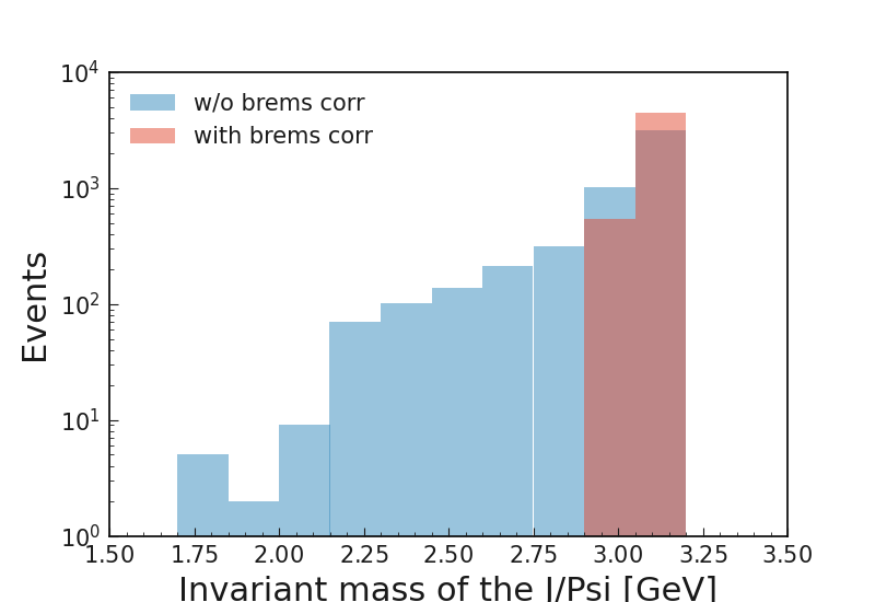
Plot a histogram of M and M_uncorrected for the correctly reconstructed $J/\psi$ mesons

Solution

#!/usr/bin/env python3

##########################################################################
# basf2 (Belle II Analysis Software Framework)                           #
# Author: The Belle II Collaboration                                     #
#                                                                        #
# See git log for contributors and copyright holders.                    #
# This file is licensed under LGPL-3.0, see LICENSE.md.                  #
##########################################################################

import matplotlib as mpl
import matplotlib.pyplot as plt
import uproot

# Only include this line if you're running from ipython an a remote server
mpl.use("Agg")

plt.style.use("belle2")  # use the official Belle II plotting style

# Declare list of variables
var_list = ['Jpsi_isSignal', 'Jpsi_M_uncorrected', 'Jpsi_M']

# Make sure that the .root file is in the same directory to find it
df = uproot.open("Bd2JpsiKS.root:tree").arrays(var_list, library='pd')

# Let's only consider signal J/Psi
df_signal_only = df.query("Jpsi_isSignal == 1")

fig, ax = plt.subplots()

ax.hist(df_signal_only["Jpsi_M_uncorrected"], label="w/o brems corr", alpha=0.5, range=(1.7, 3.2))
ax.hist(df_signal_only["Jpsi_M"], label="with brems corr", alpha=0.5, range=(1.7, 3.2))

ax.set_yscale("log")  # set a logarithmic scale in the y-axis
ax.set_xlabel("Invariant mass of the J/Psi [GeV]")
ax.set_xlim(1.5, 3.5)
ax.set_ylabel("Events")
ax.legend()  # show legend

plt.savefig("brems_corr_invariant_mass.png")

The results should look similar to Fig. 3.24 (this was obtained with a different steering file, so do not mind if your plot is not exactly the same).

../../_images/brems_corr_invariant_mass.png — Fig. 3.24 Invariant mass distributions for the reconstructed decay, $J/\psi \to e^+e^-$, with and without Bremsstrahlung correction#

Extra exercises

Store the isBremsCorrected information of the positrons and electrons used in the $J/\psi$ reconstruction
Create a variable named withBremsCorrection that indicates if any of the leptons used in the reconstruction of the B meson was Bremsstrahlung recovered

Key points

There are two ways of performing Bremsstrahlung correction: correctBrems and correctBremsBelle
Both of them create new particle lists
The members of the new particle list will have as daughter the original uncorrected particle and, if a correction was performed, the Bremsstrahlung photons used
MC matching with Bremsstrahlung corrected particles requires a special treatment: use the isSignalAcceptBremsPhotons variable, or add the ?addbrems marker in the decay string

Best Candidate Selection#

Sometimes, even after multiple selection criteria have been applied, a single event may contain more than one candidate for the reconstructed decay. In those cases, it is necessary to use some indicator that measures the quality of the multiple reconstructions, and that allow us to select the best one (or, in certain studies, select one candidate at random). Which variable to use as indicator depends on the study, and even on the analyst. Our intention here is not to tell you how to select the best quality indicator, but rather to show yo how to use it in order to select the best candidate.

The Modular Analysis package has two very useful functions, rankByHighest and rankByLowest. Each one does exactly as its name indicates: they rank particles in descending (rankByHighest) or ascending (rankByLowest) order, using the value of the variable provided as a parameter. They append to each particle an extraInfo field with the name ${variable}_rank, with the best candidate having the value one (1). Notice that each particle/anti-particle list is sorted separately, i.e., if a certain event has multiple $B^+$ and $B^-$ candidates, and you apply the ranking function to any of the particle lists, each list will be ranked separately.

Best candidate selection can then be performed by simply selecting the particle with the lowest rank. You can do that by either applying a cut on the particle list, or directly through the rankByHighest and rankByLowest functions, by specifying a non-zero value for the numBest parameter. Make sure to check the documentation of these functions.

Continuing with our example, we will make a best candidate selection using the random variable, which returns a random number between 0 and 1 for each candidate. We will select candidates with the largest value of random. In order to have uniform results across different sessions, we manually set the random seed.

Exercise

Set the basf2 random seed to "Belle II StarterKit". Then, rank your B mesons using the random variable, with the one with the highest value first. Keep only the best candidate.

Hint

You may want to check the documentation for the rankByHighest and set_random_seed functions.

Solution

# perform best candidate selection [S60]
b2.set_random_seed("Belle II StarterKit")
ma.rankByHighest("B0", variable="random", numBest=1, path=main)  # [E60]

Warning

Best candidate selection is used to pick the most adequately reconstructed decay, after all other selection cuts have been applied. As so, make sure to include it after you have performed all the other cuts in your analysis.

Exercise

Your steering file should now be complete. Run it or compare it with the solution.

Solution

#!/usr/bin/env python3

import sys
import basf2 as b2
import modularAnalysis as ma
import stdV0s
from variables import variables as vm  # shorthand for VariableManager
import variables.collections as vc
import variables.utils as vu

# get input file number from the command line
filenumber = sys.argv[1]

# create path
main = b2.Path()

# load input data from mdst/udst file
ma.inputMdstList(
    filelist=[b2.find_file(f"starterkit/2021/1111540100_eph3_BGx0_{filenumber}.root", "examples")],
    path=main,
)

# fill final state particle lists
ma.fillParticleList(
    "e+:uncorrected",
    "electronID > 0.1 and dr < 0.5 and abs(dz) < 2 and thetaInCDCAcceptance",
    path=main,
)
stdV0s.stdKshorts(path=main)

# apply Bremsstrahlung correction to electrons [S10|S20]
vm.addAlias(
    "goodFWDGamma", "passesCut(clusterReg == 1 and clusterE > 0.075)"
)  # [E10]
vm.addAlias(
    "goodBRLGamma", "passesCut(clusterReg == 2 and clusterE > 0.05)"
)
vm.addAlias(
    "goodBWDGamma", "passesCut(clusterReg == 3 and clusterE > 0.1)"
)
vm.addAlias(
    "goodGamma", "passesCut(goodFWDGamma or goodBRLGamma or goodBWDGamma)"
)  # [E20]
ma.fillParticleList("gamma:brems", "goodGamma", path=main)
ma.correctBrems("e+:corrected", "e+:uncorrected", "gamma:brems", path=main)  # [S30]
vm.addAlias("isBremsCorrected", "extraInfo(bremsCorrected)")  # [E30]

# combine final state particles to form composite particles [S40]
ma.reconstructDecay(
    "J/psi:ee -> e+:corrected e-:corrected ?addbrems",
    cut="abs(dM) < 0.11",
    path=main,
)  # [E40]

# combine J/psi and KS candidates to form B0 candidates
ma.reconstructDecay(
    "B0 -> J/psi:ee K_S0:merged",
    cut="Mbc > 5.2 and abs(deltaE) < 0.15",
    path=main,
)

# match reconstructed with MC particles
ma.matchMCTruth("B0", path=main)

# build the rest of the event
ma.buildRestOfEvent("B0", fillWithMostLikely=True, path=main)
track_based_cuts = "thetaInCDCAcceptance and pt > 0.075 and dr < 5 and abs(dz) < 10"
ecl_based_cuts = "thetaInCDCAcceptance and E > 0.05"
roe_mask = ("my_mask", track_based_cuts, ecl_based_cuts)
ma.appendROEMasks("B0", [roe_mask], path=main)

# perform best candidate selection [S60]
b2.set_random_seed("Belle II StarterKit")
ma.rankByHighest("B0", variable="random", numBest=1, path=main)  # [E60]

# Create list of variables to save into the output file
b_vars = []

standard_vars = vc.kinematics + vc.mc_kinematics + vc.mc_truth
b_vars += vc.deltae_mbc
b_vars += standard_vars

# ROE variables
roe_kinematics = ["roeE()", "roeM()", "roeP()", "roeMbc()", "roeDeltae()"]
roe_multiplicities = [
    "nROE_Charged()",
    "nROE_Photons()",
    "nROE_NeutralHadrons()",
]
b_vars += roe_kinematics + roe_multiplicities
# Let's also add a version of the ROE variables that includes the mask:
for roe_variable in roe_kinematics + roe_multiplicities:
    # e.g. instead of 'roeE()' (no mask) we want 'roeE(my_mask)'
    roe_variable_with_mask = roe_variable.replace("()", "(my_mask)")
    b_vars.append(roe_variable_with_mask)

# Variables for final states (electrons, positrons, pions)
fs_vars = vc.pid + vc.track + vc.track_hits + standard_vars
b_vars += vu.create_aliases_for_selected(
    fs_vars + ["isBremsCorrected"],
    "B0 -> [J/psi -> ^e+ ^e-] K_S0",
    prefix=["ep", "em"],
)
b_vars += vu.create_aliases_for_selected(
    fs_vars, "B0 -> J/psi [K_S0 -> ^pi+ ^pi-]", prefix=["pip", "pim"]
)
# Variables for J/Psi, KS
jpsi_ks_vars = vc.inv_mass + standard_vars
b_vars += vu.create_aliases_for_selected(jpsi_ks_vars, "B0 -> ^J/psi ^K_S0")
# Add the J/Psi mass calculated with uncorrected electrons:
vm.addAlias(  # [S50]
    "Jpsi_M_uncorrected", "daughter(0, daughterCombination(M,0:0,1:0))"
)  # [E50]
b_vars += ["Jpsi_M_uncorrected"]
# Also add kinematic variables boosted to the center of mass frame (CMS)
# for all particles
cmskinematics = vu.create_aliases(
    vc.kinematics, "useCMSFrame({variable})", "CMS"
)
b_vars += vu.create_aliases_for_selected(
    cmskinematics, "^B0 -> [^J/psi -> ^e+ ^e-] [^K_S0 -> ^pi+ ^pi-]"
)

vm.addAlias(
    "withBremsCorrection",
    "passesCut(passesCut(ep_isBremsCorrected == 1) or passesCut(em_isBremsCorrected == 1))",
)
b_vars += ["withBremsCorrection"]

# Save variables to an output file (ntuple)
ma.variablesToNtuple(
    "B0",
    variables=b_vars,
    filename="Bd2JpsiKS.root",
    treename="tree",
    path=main,
)

# Start the event loop (actually start processing things)
b2.process(main)

Extra exercises

Remove the numBest parameter from the rankByHighest function, and store both the random and the extraInfo(random_rank) variables. You can, and probably should, use aliases for these variables. Make sure that the ranking is working properly by plotting one variable against the other for events with more than one candidate (the number of candidates for a certain event is stored automatically when performing a reconstruction. Take a look at the output root file in order to find how is this variable named).
Can you think of a good variable to rank our B mesons? Try to select candidates based on this new variable, and compare how much do your results improve by, i.e., comparing the number of true positives, false negatives, or the distributions of fitting variables such as the beam constrained mass.

Note

From light release light-2008-kronos, the Modular Analysis package introduces the convenience function applyRandomCandidateSelection, which is equivalent to using rankByHighest or rankByLowest with the random variable, and with numBest equal to 1.

Key points

Best candidate selection can be performed with the rankByHighest and rankByLowest functions
These functions sort particles and antiparticles separately
From light release light-2008-kronos, a new helper function can be used to perform random candidate selection: applyRandomCandidateSelection

Stuck? We can help!

If you get stuck or have any questions to the online book material, the #starterkit-workshop channel in our chat is full of nice people who will provide fast help.

Refer to Collaborative Tools. for other places to get help if you have specific or detailed questions about your own analysis.

Improving things!

If you know how to do it, we recommend you to report bugs and other requests with GitLab. Make sure to use the documentation-training label of the basf2 project.

If you just want to give us feedback, please open a GitLab issue and add the label online_book to it.

Please make sure to be as precise as possible to make it easier for us to fix things! So for example:

typos (where?)
missing bits of information (what?)
bugs (what did you do? what goes wrong?)
too hard exercises (which one?)
etc.

If you are familiar with git and want to create your first merge request for the software, take a look at How to contribute. We’d be happy to have you on the team!

Quick feedback!

Do you want to leave us some feedback? Open a GitLab issue and add the label online_book to it.

Authors of this lesson

Alejandro Mora, Kilian Lieret

Various additions

Contents

3.4.4. Various additions#

What is Bremsstrahlung radiation?#

How do we look for Bremsstrahlung photons#

Best Candidate Selection#