Muon identification for the extrapolated tracks in KLM uses differences in longitudinal penetration depth and transverse scattering of the extrapolated track. It is handled by the Muid module, that is part of the tracking package of basf2 and proceeds in two steps:

1. Track extrapolation using the muon hypothesis only;

2. Likelihood extraction for each of six particle hypothesis: $\mu$, $\pi$, $K$, $p$, $d$, $e$.

The six likelihoods that are assigned to a given track are stored as log-likelihood values in the KLMMuidLikelihood data-object. In the post-reconstruction analysis, the log-likelihood differences may be used to select or reject the muon hypothesis for a give track.

Muid

Identifies muons by extrapolating tracks from CDC to KLM using geant4e

Package

tracking

Library

libmuid.so

14.3.1. Track extrapolation

The extrapolation proceeds step by step through the detector geometry, starting at the outermost point of the reconstructed track’s trajectory and with phase-space coordinates and covariance matrix. Upon crossing a KLM detector layer, the nearest two-dimensional hit -if any- in that layer is considered for association with the track. If the hit is within about $3.5\sigma$ (where $\sigma$ is the 2d hit uncertainty) in either of the two local-coordinates directions then it is declared a matching hit and the Kalman filter uses it to adjust the track properties before the next step in extrapolation. At the same time, the Kalman filter’s fit quality (${\chi }^2$) is accumulated for the track.

The extrapolation ends when the kinetic energy falls below a user-defined threshold (nominally 2 MeV) or the track curls inward to a cylindrical radius below the beam pipe one or the tracks escapes from KLM. If the track reached the KLM, it is classified according to how and where the extrapolation ended (stop or exited and in the barrel or the endcap).

14.3.2. Likelihood extraction

The likelihood of having the matched-hit range and transverse-scattering ${\chi }^2$ distribution is obtained from pre-calculated probability density functions (PDFs). There are separate PDFs for each charged-particle hypothesis and charge and for each extrapolation outcome.

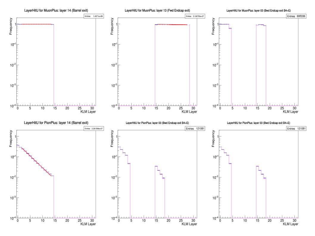
• The longitudinal-profile PDF value $P_L(\overrightarrow{x};O,l,H)$ for extrapolation ending outcome $O$ and outermost layer $l$ and for particle hypothesis $H\in {\mu }^{\pm },{\pi }^{\pm },K^{\pm },e^{\pm },p,\overline{p},d,\overline{d}$ is sampled according to the measurement vector $\overrightarrow{c}$ given by: (a) the pattern of of all KLM layers touched during the extrapolation (not just the outermost one) and (b) the pattern of matched hits in the touched layers. Sample PDF for exiting tracks are shown in Fig. 14.1 for muons and pions.

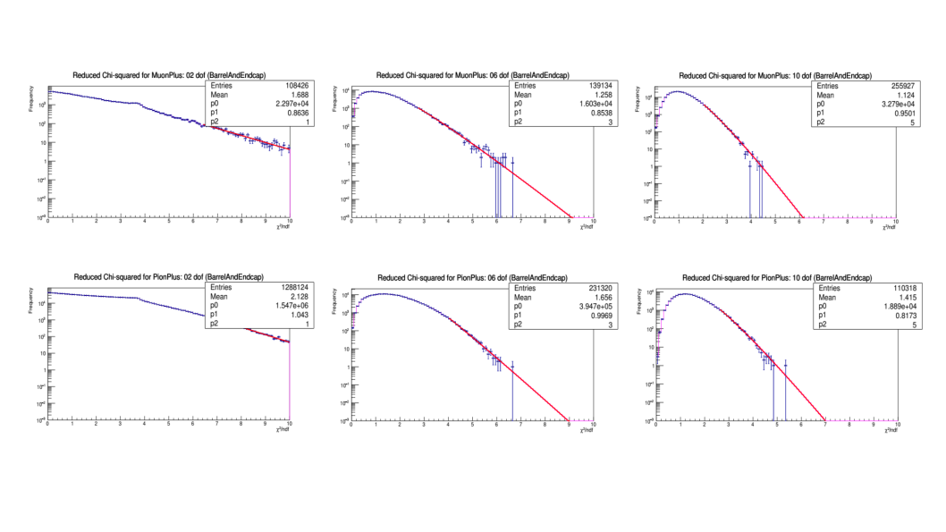
• The transverse-scattering probability density function $P_L({\chi }^2,n;D,H)$ for KLM region $D$ (barrel-only, endcap-only, or overlap) and particle hypothesis $H$ is sampled according to the measurement of ${\chi }^2$ from the Kalman filter and the number of degrees of freedom, which is twice the number of matched hits. The muon-hypothesis PDF is very close to the ideal ${\chi }^2$ distribution for the given number of degrees of freedom, while the the non-muon hypothesis PDFs are considerably broader for low degrees of freedom. Sample PDFs are shown in Fig. 14.2 for muons and pions.

Fig. 14.1 Sample longitudinal-profile PDFs for energetic positively-charged muons (top) and pions (bottom), for the barrel (left), forward endcap (middle) and a selected barrel-endcap overlap (right). The purple histogram represents the PDF. Barrel (endcap) layers are numbered 0-14 (15-28).

Fig. 14.2 Sample transverse-profile (reduced ${\chi }^2$) distributions for positively charged muons (top) and pions (bottom) for 2, 6 and 10 degrees of freedom. In each panel the red curve is the fit to the upper tail of the histogram, starting at the given cutoff.

The pre-calculated PDFs are stored in our conditions database as payload of the KLMLikelihoodParameters database object.

For each track, the likelihood for a given particle hypothesis is the product of the corresponding longitudinal-profile and transverse-scattering PDF values:

$$L(H;O,l,D,\overrightarrow{x},{\chi }^2,n)=P_L(\overrightarrow{x};O,l,H)\cdot P_T({\chi }^2,n;D,H).$$

The natural logarithm of this value is stored in the KLMMuidLikelihood data-object. Then, the six likelihood values are normalized by dividing by their sum and stored in the KLMMuidLikelihood data-object.

14.3.3. Muon Efficiency and Pion Fake Rate

The log-likelihood difference $\mathrm{\Delta }$ is the most powerful discriminator between the competing hypothesis:

$$\mathrm{\Delta }=\log (L({\mu }^{+};O,l,D,\overrightarrow{x},{\chi }^2,n))-\log (L({\pi }^{+};O,l,D,\overrightarrow{x},{\chi }^2,n)).$$

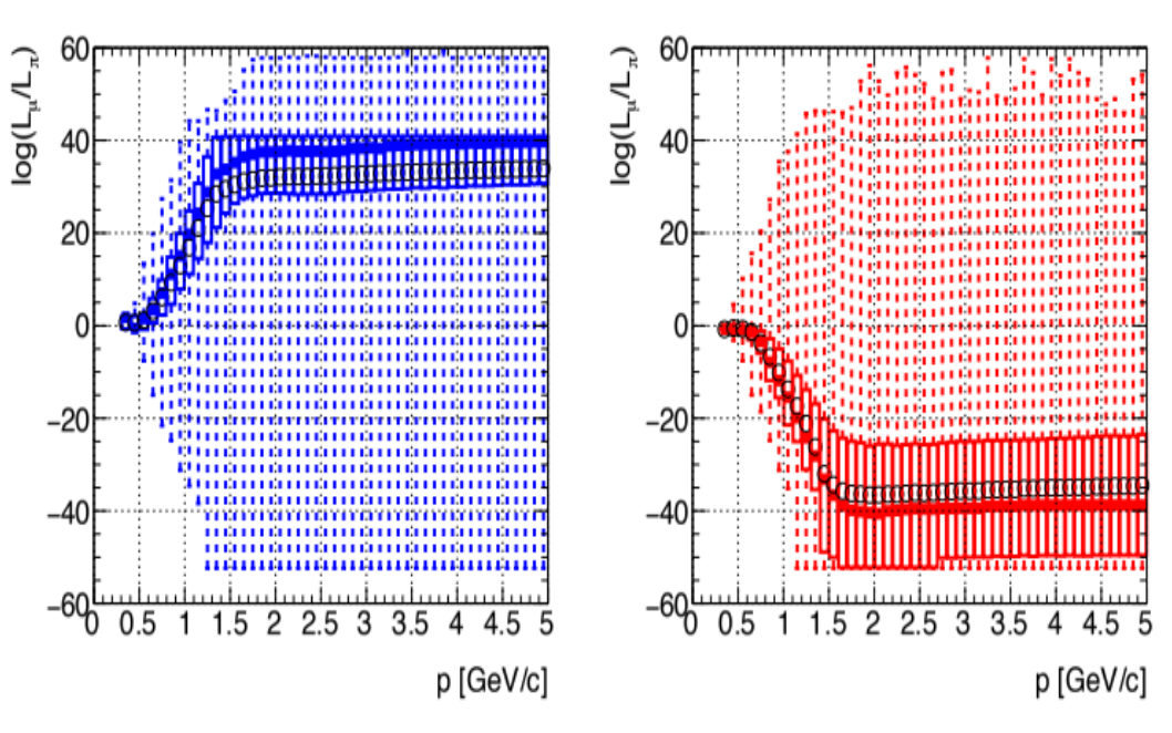
The requirement $\mathrm{\Delta }>{\mathrm{\Delta }}_{min}$ for a user-selected ${\mathrm{\Delta }}_{min}$ provides the best signal efficiency for the selected background rejection. Log-likelihood differences for true muons and pions are shown in Fig. 14.3 as a function of the track momentum. Choosing a momentum-independent cut on ${\mathrm{\Delta }}_{min}$ that is positive and non-zero will reject soft muons preferentially, and a similar behavior is seen when choosing a cut that is independent of the polar or azimuthal angles, because the log-likelihood differences are softer in the azimuthal cracks between sectors and in the barrel-endcap overlap region where KLM is thinner.

Fig. 14.3 Log-likelihood difference between muon and pion hypotheses for true muons (left) and pions (right) as a function of the track momentum in GeV/c. In each plot five features are shown: (1) minimum and maximum values (bounden by the dashed vertical line); (3) the lower and upper quartiles (below or above the rectangular box); (4)the median (the thick horizontal line segment); (5) and the mean (circle).

Muid Likelihoods are constructed by MuidBuilder class.

class MuidBuilder

Build the Muid likelihoods starting from the hit pattern and the transverse scattering in KLM.

Parameters:

• pdg (int): PDG code of the particle hypothesis.

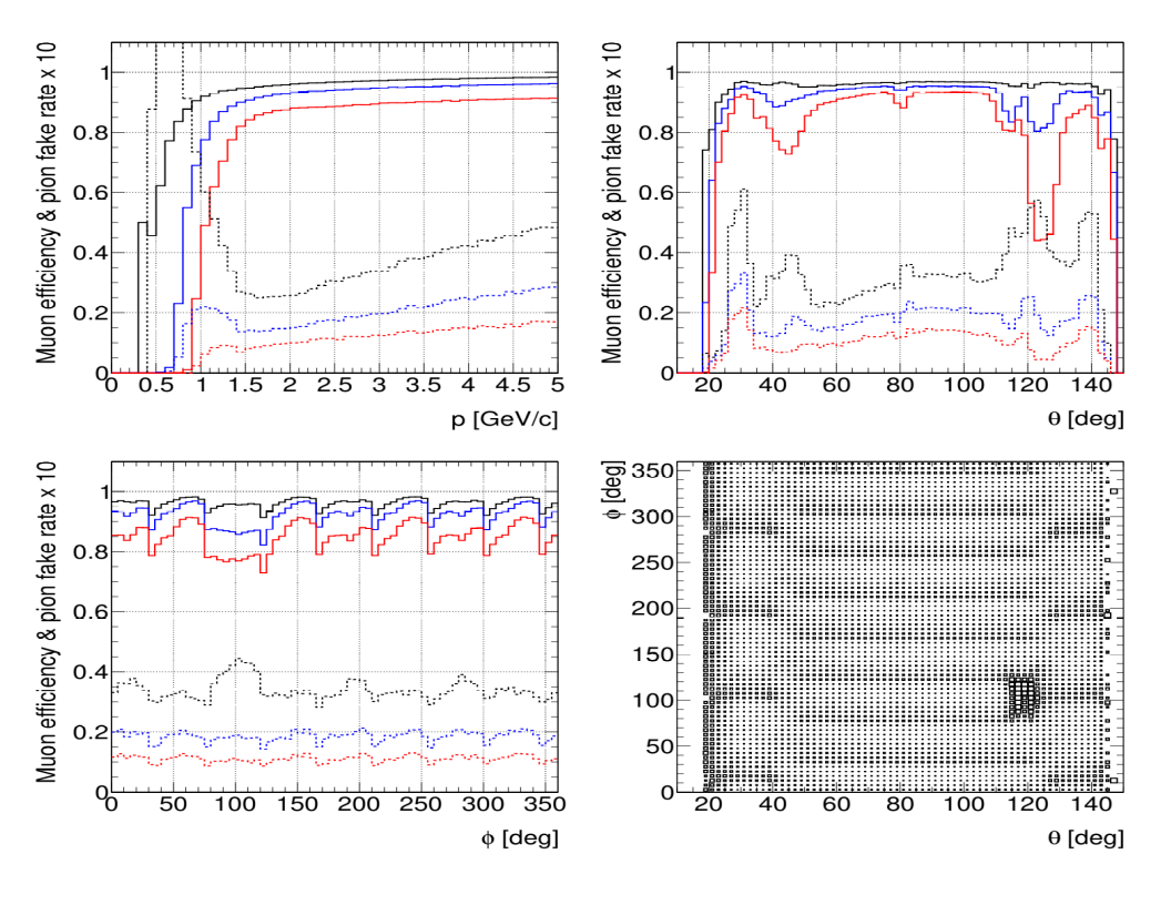
Muon efficiency and pion fake rate are shown in Fig. 14.4 as a function of momentum, polar angle, and azimuthal angle for three values of the log-likelihood-difference threshold.

Fig. 14.4 Muon efficiency (solid) and pion fake rate scaled by 10 (dashed) for three values of the log-likelihood-difference cut: ${\mathrm{\Delta }}_{min}$ = 0 (black), 10 (blue), and 20 (red) as a function of momentum (top-left), polar angle (top-right), and azimuthal angle (bottom left). Muon inefficiency as a function of $\varphi$ vs $\theta$ (bottom right), illustrating the geometric inefficiencies at the sector boundaries and in the vicinity of the solenoid chimney.

See also

“Track extrapolation and muon identification using GEANT4E in event reconstruction in the Belle II experiment”

See also

“Description and performances of the μID”