3.5.1. ROOT

If you don’t know about ROOT yet, check out the section ROOT: a nano introduction. You can find the documentation for RDataFrames here.

RDataFrames

RDataFrames are ROOT’s recommended interface to analysis. They can interpret trees in a root file into a table-like object.

import ROOT

The RDataFrame constructor takes the name of a tree and one or more files.

df = ROOT.RDataFrame("treename", "file.root")
# or
df = ROOT.RDataFrame("treename", ["file1.root", "file2.root", ...])

The location of the files can be local or remote.

To follow this tutorial, download the ntuple from https://rebrand.ly/00vvyzg (it is the same as the one in the pandas tutorial) and read it:

filepath = "pandas_tutorial_ntuple.root"
df = ROOT.RDataFrame("b0phiKs", filepath)

Inspect the contents of a tree

df.Describe()   # new in ROOT v6.26.00

Dataframe from TChain b0phiKs in file /path/to/pandas_tutorial_ntuple.root

Property                Value
--------                -----
Columns in total           50
Columns from defines        0
Event loops run             0
Processing slots            1

Column                  Type    Origin
------                  ----    ------
B0_CosTBTO              Float_t Dataset
B0_CosTBz               Float_t Dataset
B0_ErrM                 Float_t Dataset
B0_K_S0_ErrM            Float_t Dataset
B0_K_S0_M               Float_t Dataset
B0_K_S0_SigM            Float_t Dataset
B0_M                    Float_t Dataset
B0_R2                   Float_t Dataset
B0_SigM                 Float_t Dataset
B0_ThrustB              Float_t Dataset
...

Inspect the contents of one or more columns

df.Display(["B0_M", "B0_ErrM"], 5).Print()

+-----+----------+-------------+
| Row | B0_M     | B0_ErrM     |
+-----+----------+-------------+
| 0   | 5.02445f | 0.0224362f  |
+-----+----------+-------------+
| 1   | 5.10793f | 0.0823563f  |
+-----+----------+-------------+
| 2   | 5.11921f | 0.0868997f  |
+-----+----------+-------------+
| 3   | 5.36136f | 0.00969569f |
+-----+----------+-------------+
| 4   | 5.30105f | 0.00664467f |
+-----+----------+-------------+

Get the number of events in this tree

df.Count().GetValue()

Note

RDataFrames are lazy which means that operations on them are not carried out immediately, but only if a user requests it. For example, df.Count() does not return the number of events, but a Result object that promises to compute the number of events in the future. The GetValue() method extracts the actual result for us.

Functionality for data analysis

Think of an RDataFrame as a table that you can use to compute new columns from existing ones and filter based on various conditions.

df_filtered = df.Filter("condition", "optional name for this cut")

The condition can be passed either as a C++ expression in a string or as a python function. Defining new columns works in the same way:

df_new = df_filtered.Define("columnname", "c++ expression")

Note

Filter and Define do not mutate the dataframe object but rather return a new RDataFrame object. These operations are also lazy meaning that nothing is computed until the result is actually requested by the user.

For example, we could define two new columns in our RDataFrame like this:

df = df.Define("fancy_new_column", "TMath::Power((B0_deltae * B0_et), 2) / TMath::Sin(B0_cc2)")\
       .Define("delta_mbc", "B0_M - B0_mbc")

and filter it like this:

df = df.Filter("B0_mbc>5.2", "B0_mbc cut")\
       .Filter("B0_deltae>-1", "B_deltae cut")

Because of RDataFrame’s lazyness, these operations return almost instantly. The computations are only “booked”.

Exercise

Create two RDataFrames, one for Signal and one for Background only.

Hint

Split between signal and background using the B0_isSignal column.

Solution

bkgd_df = df.Filter("B0_isSignal==0")
signal_df = df.Filter("B0_isSignal==1")

Experimental new feature: Systematic variations

RDataFrames offer a declarative way to define systematic variations of columns:

nominal_df = df.Vary("pt", "ROOT::RVecD{pt*0.9, pt*1.1}", ["down", "up"])
               .Define(...)
               .Filter(...)
histo = ROOT.RDF.Experimental.VariationsFor(nominal_df)
histo["nominal"].Draw()
histo["pt:down"].Draw("SAME")

Interoperability

The columns in RDataFrames can be converted to numpy arrays for usecases where you don’t want to continue working with ROOT.

Converting to numpy is one example of the user requesting to get the data and therefore triggering the execution of all previously booked computations. You can convert one or more columns at a time:

delta_mbc = df.AsNumpy(["delta_mbc"])

We get back a dict

{'delta_mbc': ndarray([-0.18043327, -0.10750389, -0.09657669, ...,  0.02187395,
        0.04272509,  0.01566553], dtype=float32)}

and can now continue to work on the result outside of the ROOT-world.

Inspection

RDataFrames offer easily accessible methods to track down what actually happened in a computation.

For example get a report of the efficiencies of each filter applied:

df.Report().Print()

B0_mbc cut: pass=327351     all=329135     -- eff=99.46 % cumulative eff=99.46 %
B_deltae cut: pass=327349     all=327351     -- eff=100.00 % cumulative eff=99.46 %

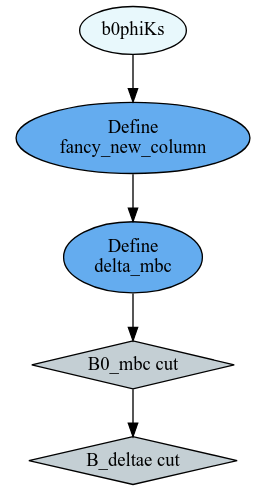
Or get the computational graph

# visualize the computation graph
ROOT.RDF.SaveGraph(df, "DAG.dot")

from graphviz import Source
Source.from_file("DAG.dot")

Scaling up

RDataFrames have the (as of now still experimental) option to run distributed on a cluster (eg. dask) to scale up your analysis.

import dask_jobqueue
from dask.distributed import Client
import ROOT
DistRDataFrame = ROOT.RDF.Experimental.Distributed.Dask.RDataFrame

cluster = dask_jobqueue.SLURMCluster(
   name="myanalysis",
   cores=1,
   queue="my-slurm-cluster",
   memory="4GB",
   job_extra_directives=[...],
)
cluster.scale(90)
client = Client(cluster)

df = DistRDataFrame("treename", filelist, daskclient=client)

Note that the interface to distributed RDataFrames is the same as normal RDataFrames, so there’s no need to change any analysis code.

Dask comes with a handy dashboard that shows the progress of all tasks across the workers, a flamegraph and many more monitoring utilities.