3.4.9. Full Event Interpretation#

Introduction#

In each ϒ(4S) decay at Belle II, two B mesons are produced. If one of the B mesons decays to a final state involving neutrinos, this B meson cannot be reconstructed completely as the neutrinos are invisible to the detector. The information can, however, be recovered from the second B meson. This is called tagging, the second B meson is referred to as B_tag. The Full Event Interpretation (FEI; pronounced like phi) is an algorithm which reconstructs this B_tag in roughly 10 000 channels. It uses a hierarchical approach to do so, first reconstructing low-level particles such as Kaons and Pions, then intermediate D mesons and finally B mesons. At each stage, the most-likely particle candidates are selected using multivariate classifiers and then used for the next stage. Usually, we do not have to train these classifiers ourselves as this requires large computing resources. Instead, the classifiers are pre-trained and can be loaded from a central database.

Fortunately, for you as a user this is all contained within a few lines of code, allowing you to easily include the FEI in your steering file. In the first part of this exercise, we will use the FEI to reconstruct a B⁺_tag and have a look at its properties. In the second part we will combine the B_tag with a B meson reconstructed in a decay channel involving neutrinos, referred to as B_sig.

Exercise

Find the documentation of the FEI and look up “hadronic tagging” and “semileptonic tagging”. What is the difference between both analysis strategies? What are advantages and disadvantages?

Hint

The documentation can be found in the Advanced Topics section of the analysis module. The definitions can be found in the section titled Hadronic, Semileptonic and Inclusive Tagging.

Solution

The documentation is here: Full event interpretation

Hadronic tagging uses only B meson decays without neutrinos and is therefore more precise (as the exact momentum of the B meson can be known).

Semileptonic tagging uses decays that include one neutrino, these have higher branching fractions but are less precise as the kinematic information is incomplete.

In this exercise we will use hadronic tagging, the procedure for semileptonic tagging is analogous but as it is less commonly used it is not discussed in this exercise.

Reconstructing a B⁺_tag#

Prerequisites#

As usual, we start our steering file by importing the necessary python packages, creating a basf2 path and loading input data. In addition to the usual python packages (basf2 and modularAnalysis) we also import the fei package.

Exercise

Import basf2, modularAnalysis and fei. In addition, we will be using variable aliases so be sure to import the variable manager. Then create a path and load input data from an mdst file.

You can again use mdst files from ${BELLE2_EXAMPLES_DATA_DIR}/starterkit/2021.

Solution

#!/usr/bin/env python3

import sys
import basf2 as b2
import fei
import modularAnalysis as ma
from variables import variables as vm

# get input file number from the command line
filenumber = sys.argv[1]

# create path
main = b2.Path()

# load input data from mdst/udst file
ma.inputMdst(
    filename=b2.find_file(f"starterkit/2021/1111540100_eph3_BGx0_{filenumber}.root", "examples"),
    path=main,
)  # [E13]

Now we need the Global Tag in which the weight files for the FEI can be found. This can change once a new central training of the FEI is released, so please check the recommended versions. One way to do so is to use the b2conditionsdb-recommend tool with the mdst file as argument. But there is also a handy method in the modularAnalysis package. Can you find it?

The correct Global Tag must then be used in your steering file by prepending it to the conditions.globaltags list in the basf2 namespace. There is also a convenience function for that!

Exercise

Include the recommended Global Tag in your steering file. For this you need to get the recommended tag using a method found in modularAnalysis and then prepend it to the list using a function documented at Conditions Database Overview.

Hint

You can get the recommended tag using modularAnalysis.getAnalysisGlobaltag

Hint

The function to prepend to the list of global tags is conditions.prepend_globaltag. Now combine this with the last hint!

Solution

Include it in the steering file like this:

# Add the database with the classifier weight files for the FEI  [S23]
b2.conditions.prepend_globaltag(ma.getAnalysisGlobaltag())  # [E23]

Configuring the FEI#

Now that all the prerequisites are there, we have to configure the FEI for our purposes. To do this, we need to configure two objects: The fei.get_default_channels function and the fei.FeiConfiguration object.

The fei.get_default_channels function controls which channels the FEI reconstructs. Disabling channels speeds up the FEI so it makes sense to only select what you need by specifying the appropriate arguments. As only charged B mesons are reconstructed in this exercise, the chargedB argument has to be set to True (default) and the neutralB argument to False. The same applies to the hadronic and semileptonic arguments, set hadronic=True and semileptonic=False as you will only reconstruct B mesons in hadronic decay channels.

B meson decay channels involving baryons are a rather new feature that increase efficiency. They are turned on by default and can be controlled with the argument baryonic.

Exercise

Configure fei.get_default_channels as described above and assign it to a variable.

Solution

# Get FEI default channels.  [S10]
# Utilise the arguments to toggle on and off certain channels
particles = fei.get_default_channels(
    chargedB=True,
    neutralB=False,
    hadronic=True,
    semileptonic=False,
    baryonic=True,
)  # [E10]

The fei.FeiConfiguration class controls the other configuration options of the FEI. Here, the FEI monitoring should be disabled with the appropriate argument (monitor=False) as we are not interested in the internal performance characteristics of the FEI stages. We also have to specify the FEI prefix argument here. This prefix allows distinguishing between different trainings in a single Global Tag and is prefix=FEIv4_2021_MC14_release_05_01_12 for the current central training.

Exercise

Configure fei.FeiConfiguration as described above and assign it to a variable.

Solution

# Set up FEI configuration specifying the FEI prefix [S20]
configuration = fei.FeiConfiguration(
    prefix="FEIv4_2021_MC14_release_05_01_12", monitor=False
)  # [E20]

The configuration created above must now be turned into a basf2 path which can be appended to the main path. This is done with the fei.get_path function which takes the channel configuration and the general FEI configuration as arguments and returns a FeiState object. The path attribute of this newly-created FeiState (e.g. feistate.path) is then appended to the main path with the basf2.Path.add_path method.

Exercise

Create the FEI path with fei.get_path() and use its basf2.Path.add_path method to add it to your main path.

Hint

The syntax is mainpath.add_path(feipath).

Solution

# Get FEI path [S30]
feistate = fei.get_path(particles, configuration)

# Add FEI path to the path to be processed
main.add_path(feistate.path)  # [E30]

You have now successfully added the FEI to the main path. The FEI will add a particle list to the datastore called B+:generic. In addition to the usual variables, the B meson candidates in the particle list will also have two extraInfo variables set: The extraInfo(decayModeID) and the extraInfo(SignalProbability) variables. The first one specifies the decay channel in which the B meson has been reconstructed, the second one is the output of the B meson classifier. This value can be used to select B meson candidates to which the FEI assigns a higher probability.

Final Steps#

What remains now is adding Monte Carlo matching and creating variable aliases for the extraInfos created by the FEI. Then, you can write the B+:generic list to a .root file. You should already be familiar with these topics from the previous exercises.

Exercise

Add MC matching to the B+:generic particle list and create variable aliases for extraInfo(decayModeID) and extraInfo(SignalProbability).

Then, write out the B+:generic particle list to a root file. Interesting variables are Mbc, deltaE, extraInfo(decayModeID), extraInfo(SignalProbability) and isSignal (or their aliases).

Finally, start the event loop with a call to basf2.process.

Hint

Go back to First steering file to see the step-by-step instructions on how to add MC matching, write the ntuple and start the event loop.

Aliases are introduced in Various additions, check there if you are unsure how to use them.

Solution

MC matching:

# Add MC matching when applying to MC. [S40]
# This is required for variables like isSignal and mcErrors below
ma.matchMCTruth(list_name="B+:generic", path=main)  # [E40]

Alias creation and output (leave out the line with FEIProbRank, this gets defined in the next exercise):

vm.addAlias("SigProb", "extraInfo(SignalProbability)")  # [S41]
vm.addAlias("decayModeID", "extraInfo(decayModeID)")

# Store tag-side variables of interest.
ma.variablesToNtuple(
    "B+:generic",
    [
        "Mbc",
        "deltaE",
        "mcErrors",
        "SigProb",
        "decayModeID",
        "FEIProbRank",
        "isSignal",
    ],
    filename="B_charged_hadronic.root",
    path=main,
)
#  [E41|E50]

The FEI returns not only one B meson candidate for each event but up to 20. Using the modularAnalysis.rankByHighest function, it is possible to rank the candidates by the B meson classifier output in the extraInfo(SignalProbability) variable. This is optional but often useful to select the best, i.e. most likely correct, candidate.

Exercise (optional)

Use rankByHighest to rank the B meson candidates in the B+:generic list by the extraInfo(SignalProbability) variable. Write the rank to a new variable called FEIProbabilityRank.

Don’t forget to create an alias for this variable (within an extraInfo metavariable) and write this to the nTuple.

Hint

You should already be familiar with Best Candidate Selection from the Various additions lesson. The documentation on rankByHighest can be found here: modularAnalysis.rankByHighest.

If the outputVariable argument of modularAnalysis.rankByHighest is called FEIProbabilityRank, the alias should be created for extraInfo(FEIProbabilityRank).

Solution

# Rank B+ candidates by signal classifier output [S50]
ma.rankByHighest(
    particleList="B+:generic",
    variable="extraInfo(SignalProbability)",
    outputVariable="FEIProbabilityRank",
    path=main,
)
vm.addAlias("FEIProbRank", "extraInfo(FEIProbabilityRank)")

vm.addAlias("SigProb", "extraInfo(SignalProbability)")  # [S41]
vm.addAlias("decayModeID", "extraInfo(decayModeID)")

# Store tag-side variables of interest.
ma.variablesToNtuple(
    "B+:generic",
    [
        "Mbc",
        "deltaE",
        "mcErrors",
        "SigProb",
        "decayModeID",
        "FEIProbRank",
        "isSignal",
    ],
    filename="B_charged_hadronic.root",
    path=main,
)
#  [E41|E50]

You can now execute your steering file which should look somewhat like this:

Final steering file

#!/usr/bin/env python3

import sys
import basf2 as b2
import fei
import modularAnalysis as ma
from variables import variables as vm

# get input file number from the command line
filenumber = sys.argv[1]

# create path
main = b2.Path()

# load input data from mdst/udst file
ma.inputMdst(
    filename=b2.find_file(f"starterkit/2021/1111540100_eph3_BGx0_{filenumber}.root", "examples"),
    path=main,
)  # [E13]

# Add the database with the classifier weight files for the FEI  [S23]
b2.conditions.prepend_globaltag(ma.getAnalysisGlobaltag())  # [E23]

# Get FEI default channels.  [S10]
# Utilise the arguments to toggle on and off certain channels
particles = fei.get_default_channels(
    chargedB=True,
    neutralB=False,
    hadronic=True,
    semileptonic=False,
    baryonic=True,
)  # [E10]
# Set up FEI configuration specifying the FEI prefix [S20]
configuration = fei.FeiConfiguration(
    prefix="FEIv4_2021_MC14_release_05_01_12", monitor=False
)  # [E20]

# Get FEI path [S30]
feistate = fei.get_path(particles, configuration)

# Add FEI path to the path to be processed
main.add_path(feistate.path)  # [E30]

# Add MC matching when applying to MC. [S40]
# This is required for variables like isSignal and mcErrors below
ma.matchMCTruth(list_name="B+:generic", path=main)  # [E40]

# Rank B+ candidates by signal classifier output [S50]
ma.rankByHighest(
    particleList="B+:generic",
    variable="extraInfo(SignalProbability)",
    outputVariable="FEIProbabilityRank",
    path=main,
)
vm.addAlias("FEIProbRank", "extraInfo(FEIProbabilityRank)")

vm.addAlias("SigProb", "extraInfo(SignalProbability)")  # [S41]
vm.addAlias("decayModeID", "extraInfo(decayModeID)")

# Store tag-side variables of interest.
ma.variablesToNtuple(
    "B+:generic",
    [
        "Mbc",
        "deltaE",
        "mcErrors",
        "SigProb",
        "decayModeID",
        "FEIProbRank",
        "isSignal",
    ],
    filename="B_charged_hadronic.root",
    path=main,
)
#  [E41|E50]
# Process events
b2.process(main)
print(b2.statistics)

Offline analysis#

Now that you have created your ntuple, we can have a look at the properties of the B mesons we have created.

You have already looked at the beam-constrained mass Mbc in First steering file. For correctly reconstructed B mesons, this variable should peak at the B meson mass. It is therefore a good indicator for the quality of the B mesons we have reconstructed.

Exercise

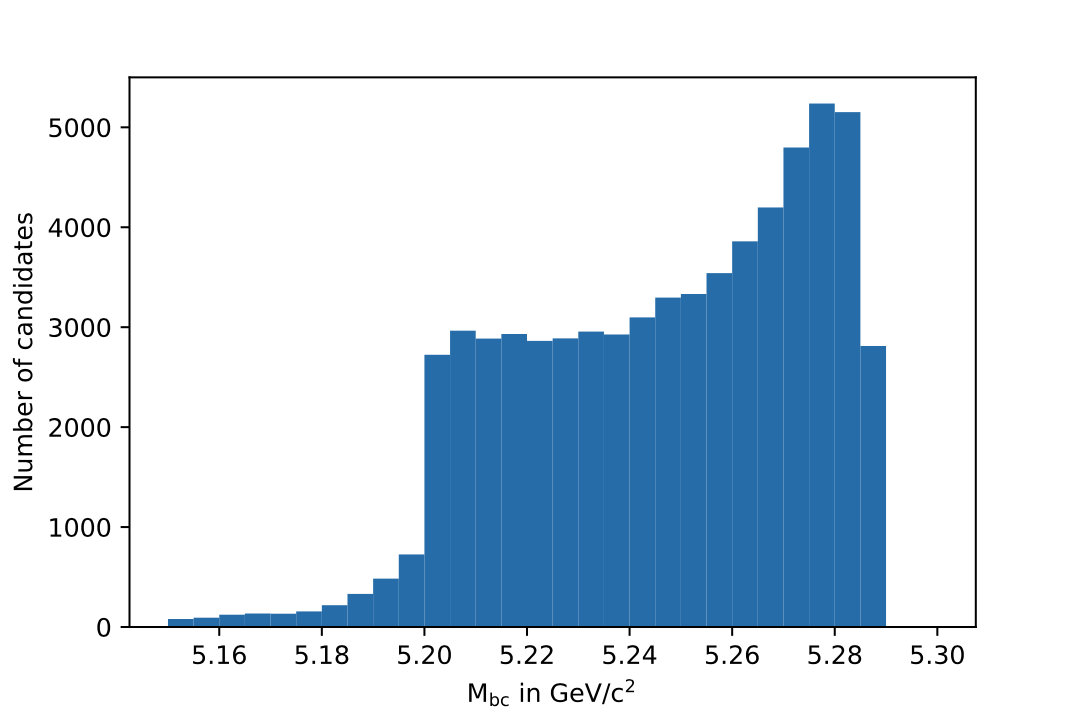
Load your ntuple file into python, either using root_pandas or uproot. The latter is strongly recommended since root_pandas is deprecated and unmaintained. For instructions on the basic usage of uproot see the Getting started guide. After loading your ntuple, plot the distribution of Mbc from 5.15 – 5.3 GeV.

You should see broad peak with a sharp drop-off below 5.2 GeV. This drop-off is caused by a fixed pre-cut in the FEI. Candidates below this threshold are rejected before classification as they are almost always incorrect.

Solution

# Include this only if running in a Jupyter notebook
%matplotlib inline

import matplotlib.pyplot as plt
import uproot

# To load a root tree with uproot.open, the argument has to be in the form 'filename:treename'
df = uproot.open('B_charged_hadronic.root:variables').arrays(['Mbc'], library='pd')

fig, ax = plt.subplots()
n, bins, patches = ax.hist(df['Mbc'], bins=30, range=(5.15, 5.3))
ax.set_xlabel(r'$\mathrm{M}_{\mathrm{bc}}$ in GeV/c$^2$')
ax.set_ylabel('Number of candidates')
fig.savefig('m_bc.pdf')

Question

The distribution of Mbc you have just plotted doesn’t peak at the B meson mass of 5.28 GeV. Can you explain this?

Solution

We haven’t really used the classifier output of the FEI yet. The up to 20 candidates in each event are selected by FEI Signal Probability but many still have low absolute classifier values and by definition almost all of them are misreconstructed.

Exercise

Increase the signal purity by requiring minimum values of extraInfo__boSignalProbability__bc. Try cuts at 0.001, 0.01 and 0.1!

You can also try selecting the candidate with the highest FEI Probability in each event by using the extraInfo__boFEIProbabilityRank__bc variable created with modularAnalysis.rankByHighest (if you have done this).

These selections should increase the purity of the B meson candidates under consideration and lead to a sharper peak at the B mass.

You can also have a look at the correctly reconstructed B mesons by requiring isSignal == 1. By comparing this to the cuts on the FEI classifier you can see how well the FEI identifies correctly reconstructed B mesons.

Solution

# Include this only if running in a Jupyter notebook
%matplotlib inline

import matplotlib.pyplot as plt
import uproot

df = uproot.open('B_charged_hadronic.root:variables').arrays(['Mbc', 'SigProb', 'FEIProbRank'], library='pd')

fig, ax = plt.subplots()

# If you didn't do the optional exercise, the 'FEIProbRank' column won't be there.
# Just remove this part of the query in this case.
sig_prob_cut_df = df.query('(SigProb > 0.01) & (FEIProbRank == 1)')

n, bins, patches = ax.hist(sig_prob_cut_df['Mbc'], bins=30, range=(5.15, 5.3))
ax.set_xlabel(r'$\mathrm{M}_{\mathrm{bc}}$ in GeV/c$^2$')
ax.set_ylabel('Total number of candidates')
ax.set_title('SigProb > 0.01')
fig.savefig('m_bc_cut_0_01.pdf')

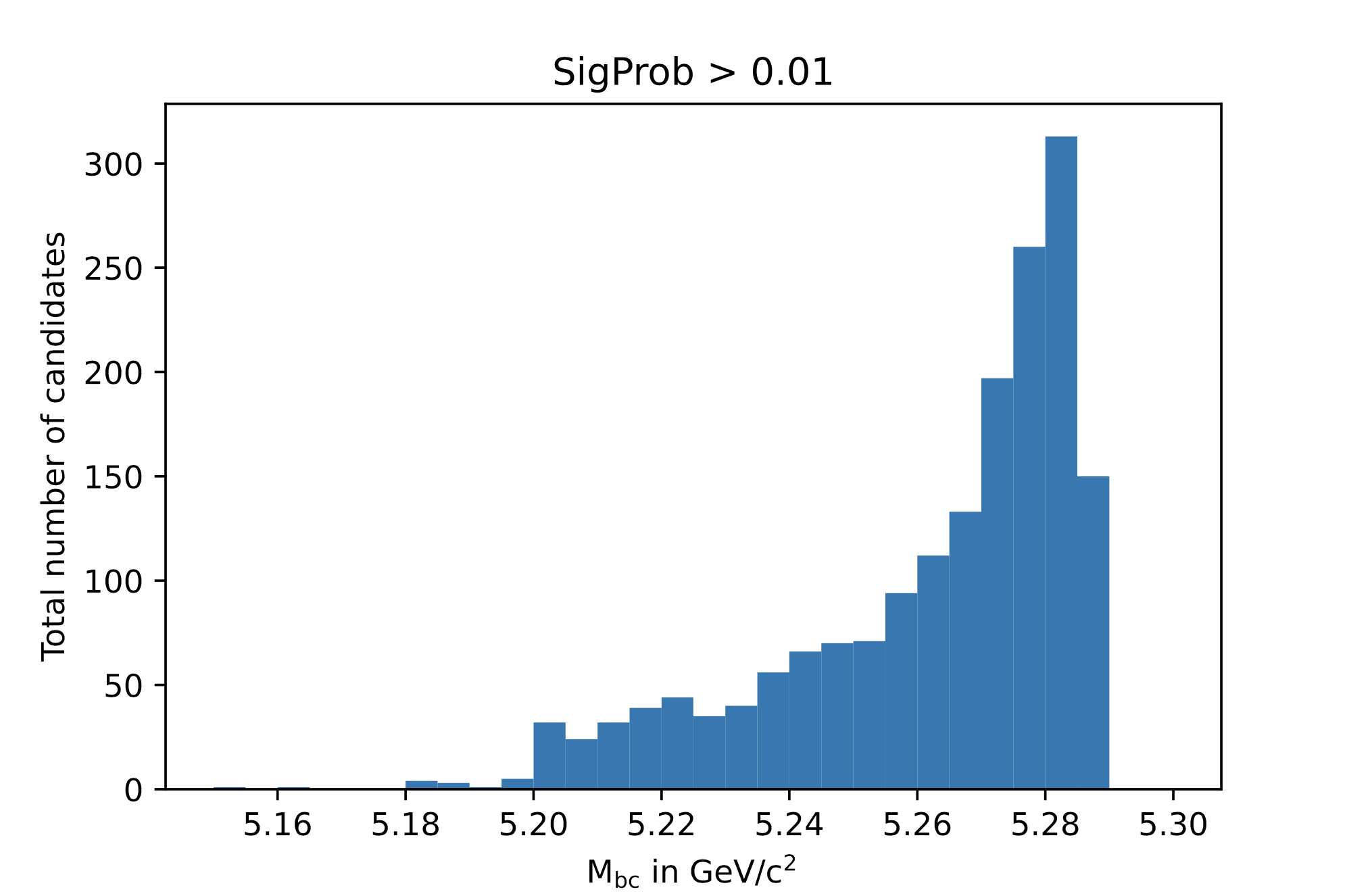
Congratulations, you have now discovered the B meson in Monte Carlo data! This concludes the first part of this lesson. The second part of this lesson will show you now how to use the reconstructed B_tag in your own analysis.

Reconstructing the full ϒ(4S) event#

In this part of the lesson, we will reconstruct the full ϒ(4S) event using the FEI. The B⁰ decay process we will be looking at is the semileptonic decay to a charged pion, a muon and a muon neutrino.

The FEI skim#

You might have noticed that applying the FEI takes some time, even for the small file we have just processed. For this reason and to save computing resources, datasets with pre-applied FEI tagging exist. These preprocessed datasets are called skims.

We will be using a FEI-skimmed file in this exercise in which the B0:generic particle list already exists. If you would like to know more about skimming, you can have a look into Skimming.

The input file we will be using, found at ${BELLE2_EXAMPLES_DATA_DIR}/starterkit/2021/fei_skimmed_xulnu.udst.root, only contains decays of B0 mesons to a light lepton and a charged pi or rho meson. This way we don’t have to process as much data as we would have to for a file containing decays in all B decay channels.

Prerequisites (part 2)#

Lets get started with the usual steps. Nothing here should be new to you.

Exercise

Start a new steering file. In this file, you won’t need the fei package so you can skip this import. Create a path and load the udst file ${BELLE2_EXAMPLES_DATA_DIR}/starterkit/2021/fei_skimmed_xulnu.udst.root.

NOTE: You can still use modularAnalysis.inputMdst to do this, even though it’s a udst file.

Then, fill two particle lists with muons and charged pions. For the muons, you can require a muonID above 0.9, for the pions a pionID above 0.5. For both you should apply some requirements on the track, you can use dr < 0.5 and abs(dz) < 2 and nCDCHits > 20 and thetaInCDCAcceptance

Hint

You should already be familiar with this from First steering file.

Solution

#!/usr/bin/env python3

import basf2 as b2
import modularAnalysis as ma
from variables import variables as vm

main = b2.Path()

ma.inputMdst(
    filename=b2.find_file("starterkit/2021/fei_skimmed_xulnu.udst.root", "examples"),
    path=main,
)

good_track = (
    "dr < 0.5 and abs(dz) < 2 and nCDCHits > 20 and thetaInCDCAcceptance"
)

ma.fillParticleList("mu-", "muonID > 0.9 and " + good_track, path=main)
ma.fillParticleList("pi-", "pionID > 0.5 and " + good_track, path=main)  # [E60]

ϒ(4S) Reconstruction#

Now, let’s get started with the reconstruction. We will first create the signal B meson, then combine it with the B meson provided by the FEI to get the ϒ(4S).

As the semileptonic decay we are analysing contains a neutrino, a few things have to be considered. The neutrino is not used the reconstruction of the B_sig as it can’t be seen in the Belle II detector. This leads to a discrepancy between the simulated decay and the reconstructed decay, causing the isSignal variable to always be zero.

To solve this you can tell the MC matching algorithm to accept missing neutrinos by using the ?nu flag, similar to the ?addbrems flag introduced in Various additions. Just add this flag to the end of the decay string in modularAnalysis.reconstructDecay. 1

Exercise

Reconstruct a B⁰ meson particle list called B0:signal from a positive pion and a muon. Add the ?nu flag as described above.

Solution

ma.reconstructDecay("B0:signal -> pi- mu+ ?nu", cut="", path=main)  # [S113|E113]

So far, we have not used the FEI. Now, we will use the B_tag in the udst file and combine it with the B_sig we have just created.

Exercise

Combine the B0:generic from the udst file with the anti-B0:signal to a list called Upsilon(4S):opposite_cp .

NOTE: The B0:generic should come first in the decay string, otherwise the missing mass squared variable we’re using later won’t know which of the B mesons is the tag and which is the signal.

Can you think of a reason for the opposite_cp identifier of the Upsilon(4S) list?

Have we forgotten something?

Hint

Think of special properties of B⁰ mesons compared to B⁺ mesons.

For the implementation: You will most likely need one more modularAnalysis.reconstructDecay to create the second particle list and the modularAnalysis.copyLists function to combine both lists.

Solution

To account for B⁰ meson mixing, you should also combine same-sign B⁰ mesons as the anti-B⁰ can oscillate to a B⁰.

ma.reconstructDecay(  # [S70]
    "Upsilon(4S):opposite_cp -> B0:generic anti-B0:signal", cut="", path=main
)
ma.reconstructDecay(
    decayString="Upsilon(4S):same_cp -> B0:generic B0:signal",
    cut="",
    path=main,
)
# Combine the two Upsilon(4S) lists to one. Note: Duplicates are removed.
ma.copyLists(
    outputListName="Upsilon(4S)",
    inputListNames=["Upsilon(4S):opposite_cp", "Upsilon(4S):same_cp"],
    path=main,
)  # [E70]

Now that we have reconstructed the full ϒ(4S), we will create a Rest of Event. You have already done this in The Rest of Event (ROE) for a B meson, here however we will create a Rest of Event for the ϒ(4S). This allows us to count the tracks left over after reconstructing the ϒ(4S), for two correctly reconstructed B mesons there should be no tracks left over.

For this to work we have to use a slightly different ROE mask than in the ROE chapter. To match the cuts used by the FEI to reconstruct B_tag candidates, we have to tighten the cut on dr to below 2 and the cut on the absolute value of dz (abs(dz)) to below 4. The two other cuts (on pt and thetaInCDCAcceptance) can be left as-is.

Exercise

Create a Rest of Event for the Upsilon(4S) list. Then, append an ROE mask using the cuts introduced in the chapter The Rest of Event (ROE) and the additional track cuts mentioned above.

Hint

The track cuts should be thetaInCDCAcceptance and pt > 0.075 and dr < 2 and abs(dz) < 4 and the ecl cuts thetaInCDCAcceptance and E > 0.05. To create the ROE, use modularAnalysis.buildRestOfEvent. To append the ROE mask, use modularAnalysis.appendROEMasks.

Solution

ma.buildRestOfEvent("Upsilon(4S)", path=main)  # [S80]
track_based_cuts = "thetaInCDCAcceptance and pt > 0.075 and dr < 2 and abs(dz) < 4"
ecl_based_cuts = "thetaInCDCAcceptance and E > 0.05"
roe_mask = ("my_mask", track_based_cuts, ecl_based_cuts)
ma.appendROEMasks("Upsilon(4S)", [roe_mask], path=main)  # [E80]

Writing out the nTuple#

We are now ready to add MC matching and write out the nTuple.

While the MC matching is applied to the Upsilon(4S) list, you can also access the daughter’s truth variables using the daughter metavariable.

This is especially useful in FEI analyses:

As you might have noticed in the first part of the exercise, the number of perfectly (i.e. isSignal == 1.0) reconstructed B_tag mesons is not very large As we are only really interested in the B_sig, the isSignal variable of this B meson can be a better signal definition than the isSignal variable of the Upsilon(4S)

In addition to the properties of the B mesons, we can now also use information from the full event.

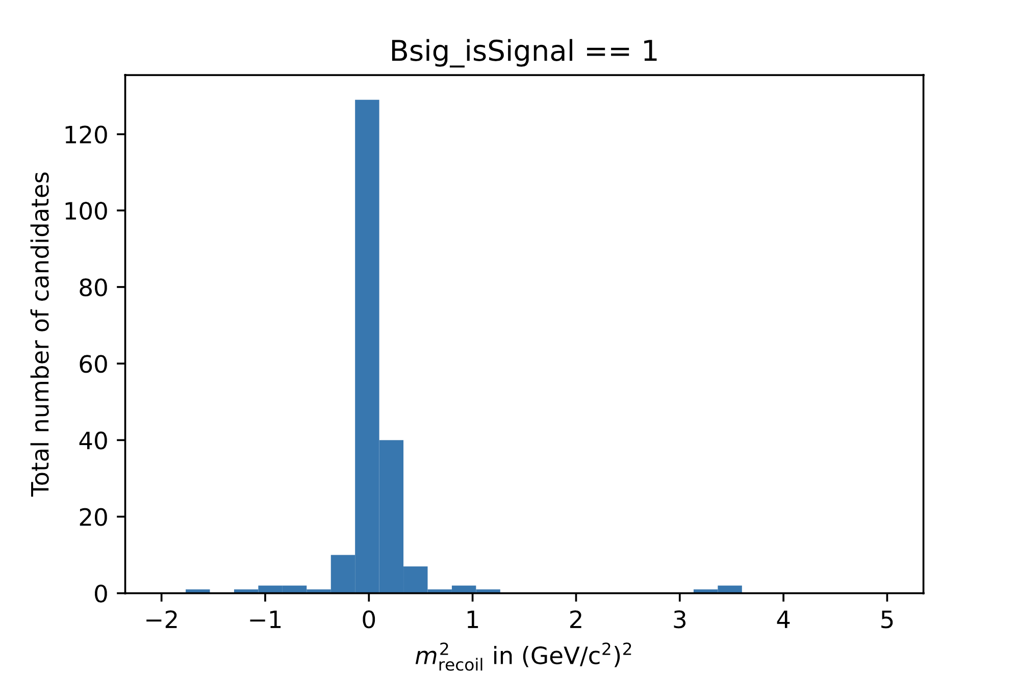
An example here is the missing mass squared in the variable m2RecoilSignalSide. This quantity should peak at zero for decays in which only one neutrino is missing and thus provides high separating power in (semi-)leptonic analyses. There are different implementations of the missing mass squared in basf2, this version uses the explicit B_tag momentum (here reconstructed by the FEI) and has therefore a high resolution.

A second variable with high separating power is the number of additional charged tracks introduced above. This variable is called nROE_Charged in basf2. It needs the ROE mask name defined above as an argument in brackets.

Exercise

Add MC matching for the Upsilon(4S) to your path.

Write the Upsilon(4S) particle list to an nTuple. Include the variables used in the first part of the lesson, the signal variables mentioned above (both for the B_sig and the ϒ(4S)), the missing mass squared and the number of additional tracks.

It is recommended to define aliases for the variables as otherwise the variables will be long and unwieldy in your offline analysis.

Finally, don’t forget to process the path!

Hint

If you have forgotten how to use aliases: This is introduced in Various additions.

If you have adapted the solution given here, the variable containing the number of additional tracks will be nROE_Charged(my_mask).

Solution

ma.matchMCTruth(list_name="Upsilon(4S)", path=main)  # [S90]

vm.addAlias("Btag_SigProb", "daughter(0, extraInfo(SignalProbability))")
vm.addAlias("Btag_decayModeID", "daughter(0, extraInfo(decayModeID))")
vm.addAlias("Btag_Mbc", "daughter(0, Mbc)")

vm.addAlias("Bsig_isSignal",
            "daughter(1, isSignal)")
vm.addAlias("nCharged", "nROE_Charged(my_mask)")

ma.variablesToNtuple(
    "Upsilon(4S)",
    variables=[
        "Btag_SigProb",
        "Btag_decayModeID",
        "Btag_Mbc",
        "Bsig_isSignal",
        "isSignal",
        "m2RecoilSignalSide",
        "nCharged"
    ],
    filename='Upsilon4S.root',
    path=main,
)
# Process events
b2.process(main)  # [E90]

You can now execute your steering file which should look somewhat like this:

Final steering file

#!/usr/bin/env python3

import basf2 as b2
import modularAnalysis as ma
from variables import variables as vm

main = b2.Path()

ma.inputMdst(
    filename=b2.find_file("starterkit/2021/fei_skimmed_xulnu.udst.root", "examples"),
    path=main,
)

good_track = (
    "dr < 0.5 and abs(dz) < 2 and nCDCHits > 20 and thetaInCDCAcceptance"
)

ma.fillParticleList("mu-", "muonID > 0.9 and " + good_track, path=main)
ma.fillParticleList("pi-", "pionID > 0.5 and " + good_track, path=main)  # [E60]

ma.reconstructDecay("B0:signal -> pi- mu+ ?nu", cut="", path=main)  # [S113|E113]

ma.reconstructDecay(  # [S70]
    "Upsilon(4S):opposite_cp -> B0:generic anti-B0:signal", cut="", path=main
)
ma.reconstructDecay(
    decayString="Upsilon(4S):same_cp -> B0:generic B0:signal",
    cut="",
    path=main,
)
# Combine the two Upsilon(4S) lists to one. Note: Duplicates are removed.
ma.copyLists(
    outputListName="Upsilon(4S)",
    inputListNames=["Upsilon(4S):opposite_cp", "Upsilon(4S):same_cp"],
    path=main,
)  # [E70]

ma.buildRestOfEvent("Upsilon(4S)", path=main)  # [S80]
track_based_cuts = "thetaInCDCAcceptance and pt > 0.075 and dr < 2 and abs(dz) < 4"
ecl_based_cuts = "thetaInCDCAcceptance and E > 0.05"
roe_mask = ("my_mask", track_based_cuts, ecl_based_cuts)
ma.appendROEMasks("Upsilon(4S)", [roe_mask], path=main)  # [E80]

ma.matchMCTruth(list_name="Upsilon(4S)", path=main)  # [S90]

vm.addAlias("Btag_SigProb", "daughter(0, extraInfo(SignalProbability))")
vm.addAlias("Btag_decayModeID", "daughter(0, extraInfo(decayModeID))")
vm.addAlias("Btag_Mbc", "daughter(0, Mbc)")

vm.addAlias("Bsig_isSignal",
            "daughter(1, isSignal)")
vm.addAlias("nCharged", "nROE_Charged(my_mask)")

ma.variablesToNtuple(
    "Upsilon(4S)",
    variables=[
        "Btag_SigProb",
        "Btag_decayModeID",
        "Btag_Mbc",
        "Bsig_isSignal",
        "isSignal",
        "m2RecoilSignalSide",
        "nCharged"
    ],
    filename='Upsilon4S.root',
    path=main,
)
# Process events
b2.process(main)  # [E90]
print(b2.statistics)

Offline analysis (part 2)#

Like in the first part of this lesson, you can now analyse your nTuple. As before, you can use the FEI signal probability (now under the alias Btag_SigProb if you have adapted the example) to select more pure ϒ(4S) candidates and plot m2RecoilSignalSide for different values of the classifier.

You can also see how cuts on the number of additional tracks change the histogram.

NOTE: A histogram of Mbc will look quite different in this part of the exercise, this is because in the last exercise we have used a generic MC sample and in this exercise we are using an MC sample with only four decay channels.

Exercise

Plot m2RecoilSignalSide for Bsig_isSignal == 1.0 to see what well-reconstructed B -> pi l nu decays should look like. Then, plot m2RecoilSignalSide for different cuts on the FEI classifier output. See also how the shape of m2RecoilSignalSide changes when requiring zero additional tracks.

Solution

# Include this only if running in a Jupyter notebook
%matplotlib inline

import matplotlib.pyplot as plt
import uproot

df = uproot.open('Upsilon4S.root:variables').arrays(['Bsig_isSignal',
                                                     'm2RecoilSignalSide',
                                                     'Btag_SigProb',
                                                     'nCharged'],
                                                    library='pd')

fig, ax = plt.subplots()

# Requiring only the B_sig to be correctly reconstructed.
# Try what happens if you require the whole Y(4S) to be correct!
signal_df = df.query('(Bsig_isSignal  == 1.0)')

n, bins, patches = ax.hist(signal_df['m2RecoilSignalSide'], bins=30, range=(-2, 5))
ax.set_xlabel(r'$m^2_{\mathrm{recoil}}$ in (GeV/c$^2$)$^2$')
ax.set_ylabel('Total number of candidates')
ax.set_title('Bsig_isSignal == 1')
fig.savefig('m2RSS_Signal.pdf')

fig, ax = plt.subplots()

# This is just an example cut, you can try without the cut on nCharged
# and for different values on BtagSigProb
cut_df = df.query('(Btag_SigProb > 0.01) & (nCharged == 0.0)')

n, bins, patches = ax.hist(cut_df['m2RecoilSignalSide'], bins=30, range=(-2, 5))
ax.set_xlabel(r'$m^2_{\mathrm{recoil}}$ in (GeV/c$^2$)$^2$')
ax.set_ylabel('Total number of candidates')
ax.set_title('SigProb > 0.01')
fig.savefig('m2RSS_FEIcut_0_01_nCharged_0.pdf')

../../_images/m2RSS_FEIcut_0_01_nCharged_0.png

Congratulations, you now know how to run the FEI and how to use it in your analysis. If you would like to know more you can always read the extensive documentation of the FEI. Here you can also find instructions on how to train the FEI and explanations on the code structure.

Key points

Get the weight files from the conditions database
Add the FEI to your path with fei.get_default_channels and fei.FeiConfiguration.
FEI Purity and efficiency are controlled by a cut on extraInfo(SignalProbability)
The B_tag from the FEI can be used to construct a complete ϒ(4S) event.

Stuck? We can help!

If you get stuck or have any questions to the online book material, the #starterkit-workshop channel in our chat is full of nice people who will provide fast help.

Refer to Collaborative Tools. for other places to get help if you have specific or detailed questions about your own analysis.

Improving things!

If you know how to do it, we recommend you to report bugs and other requests with GitLab. Make sure to use the documentation-training label of the basf2 project.

If you just want to give very quick feedback, use the last box “Quick feedback”.

Please make sure to be as precise as possible to make it easier for us to fix things! So for example:

typos (where?)
missing bits of information (what?)
bugs (what did you do? what goes wrong?)
too hard exercises (which one?)
etc.

If you are familiar with git and want to create your first merge request for the software, take a look at How to contribute. We’d be happy to have you on the team!

Quick feedback!

Author of this lesson

Moritz Bauer

Footnotes

1: Alternatively, you can also use the isSignalAcceptMissingNeutrino variable instead of isSignal but we will be going with the ?nu flag and isSignal in our example.

basf2 development documentation

Full Event Interpretation

Contents

3.4.9. Full Event Interpretation#

Introduction#

Reconstructing a B⁺_tag#

Prerequisites#

Configuring the FEI#

Final Steps#

Offline analysis#

Reconstructing the full ϒ(4S) event#

The FEI skim#

Prerequisites (part 2)#

ϒ(4S) Reconstruction#

Writing out the nTuple#

Offline analysis (part 2)#

basf2 development documentation

Full Event Interpretation

Contents

3.4.9. Full Event Interpretation#

Introduction#

Reconstructing a B+tag#

Prerequisites#

Configuring the FEI#

Final Steps#

Offline analysis#

Reconstructing the full ϒ(4S) event#

The FEI skim#

Prerequisites (part 2)#

ϒ(4S) Reconstruction#

Writing out the nTuple#

Offline analysis (part 2)#

Reconstructing a B⁺_tag#