
3.5.6. Topology analysis#
Tip
This online textbook introduces TopoAna very briefly.
For more descriptions of the tool, please refer to the documents introduced
in Section 7.7.9.
Please feel free to contact Xingyu Zhou (zhouxy@buaa.edu.cn) if you have any
questions or comments on TopoAna and this online textbook.
Introduction#
In the data analysis of high energy physics experiments, a comprehensive understanding of the inclusive/generic MC samples is required to select signals with a higher efficiency and meanwhile suppress backgrounds to a lower level. In particular, a clear knowledge of the physics processes, namely the event types, involved in the samples is quite helpful.
With the physics process information, we can figure out the main backgrounds (especially the peaking ones). Then, we can optimize the selection criteria further by analyzing the differences between the main backgrounds and the signals. Even if it is difficult to further suppress these backgrounds, the knowledge of their types is beneficial to estimate the systematic uncertainties associated with them.
Sometimes, we need to search for certain processes of interests. Mostly, signal and background events coexist in inclusive MC samples. It is useful to differentiate them in such cases. The identified signal events can be used to make up a signal sample in the absence of specialized signal samples, or they can be removed to avoid repetition in the presence of specialized signal samples. Occasionally, we have to pick out some decay branches in order to re-weight them according to new theoretical predictions or updated experimental measurements.
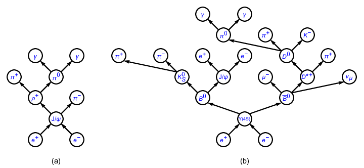
Fig. 3.30 Topology diagrams of (a) \(e^+ e^- \to J/\psi\), \(J/\psi \to \rho^+ \pi^-\), \(\rho^+ \to \pi^+ \pi^0\), \(\pi^0 \to \gamma \gamma\) and (b) \(e^+ e^- \to \Upsilon(4S)\), \(\Upsilon(4S) \to B^0 \bar{B}^0\), \(B^0 \to K_S^0 J/\psi\), \(\bar{B}^0 \to \mu^- D^{*+} \nu_{\mu}\), \(K_S^0 \to \pi^+ \pi^-\), \(J/\psi \to e^+ e^-\), \(D^{*+} \to D^0 \pi^+\), \(D^0 \to \pi^0 \pi^+ K^-\), \(\pi^0 \to \gamma \gamma\).#
Processes in high energy physics can be visualized with topology diagrams. As an example, Fig. 3.30 shows the topology diagrams of two typical physics processes occurring at \(e^+e^-\) colliders. From the figure, the hierarchies of the processes and the relationships among the particles are clearly illustrated with the diagrams. Though the complexities of topology diagrams vary with physics processes, there is only one diagram corresponding to each process. For this reason, we refer to the physics process information/analysis mentioned thereinbefore as topology information/analysis hereinafter.
Since the raw topology truth information of inclusive MC samples is counter-intuitive,
diverse, and overwhelming, it is difficult for analysts to check the topology
information of the samples directly.
To help them do the checks quickly and easily, a topology analysis program called
TopoAna is developed with C++, ROOT, and LaTeX.
Basics of the program#
The input of the program is one or more root files including a TTree object
which contains the raw topology truth information of the inclusive MC samples
under study.
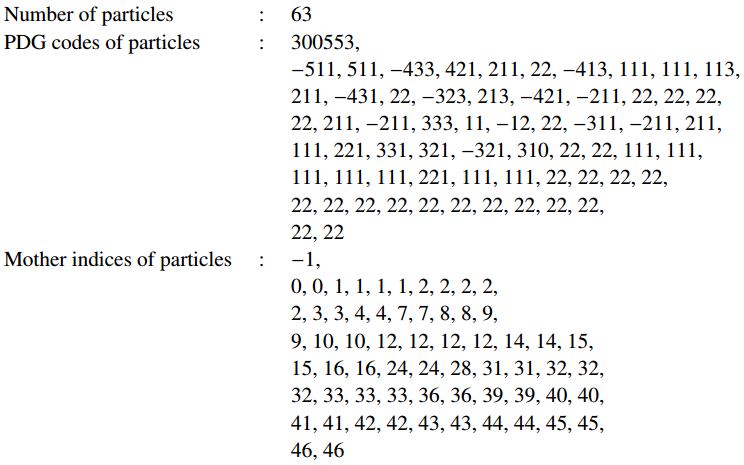
To be specific, the information in each entry of the TTree object consists
of the following three ingredients associated with the particles produced in an
event of the samples: the number of the particles, the PDG codes of the
particles, and the mother indices of the particles.
Note
The particles do not include the initial state particles (\(e^+\) and \(e^-\) in the Belle II experiment), which are default and thus omitted.
The indices of particles are integers starting from zero (included) to the number of particles (excluded); they are obvious and hence not taken as an input ingredient for topology analysis.
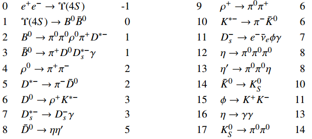
Fundamentally, the program resolves counter-intuitive, diverse, and overwhelming input data
into highly readable symbolic expressions of physics processes
Tip
Here, the decay branches in the process are placed into two blocks in order to make full use of the page space.
In both blocks, the first, second, and third columns are the indices, symbolic expressions, and mother indices of the decay branches.
Notably, all the decay branches of \(\pi^0 \to \gamma \gamma\) are omitted in order to make the process look more concise.
Generally, the functionalities of the program are as follows.
The program recognizes, categorizes, and counts physics processes in each event of the samples.
It tags the physics processes in the corresponding entry of the output root files.
Tip
Except for the tags, the input
TTreeobject in the output root files is entirely the same as that in the input root files.After processing the events, the program exports the obtained topology information at the sample level (topology maps) to the output plain text, tex source, and pdf files.
Tip
Although the files are in different formats, they have the same information.
The pdf file is the easiest to read. It is converted from the tex source file by the
pdflatexcommand.The plain text file is convenient to be checked with text processing commands as well as text editors.
Note
Below are some general remarks on the relationship between the TopoAna
program and the MC matching module in basf2, namely
MCMatcherParticles.
As we introduce in Section 7.7.9,
TopoAnais an offline tool independent ofbasf2. It gets the human-friendly topology information on its own from the raw MC truth information obtained with the interfaceMCGenTopo. Obviously, it does not rely onMCMatcherParticles.On the other hand, in order to analyze some backgrounds more effectively, a series of newly developed parameters in a few functionality items in
TopoAnacan make use of the MC matching results obtained withMCMatcherParticles. For more details, please see Section 5.2.3 (titled Reconstruction restrictions on truth particles) in the user guide we introduce in Section 7.7.9.In addition, there are some functionality overlaps between
TopoAnaandMCMatcherParticles. If highly needed, in the future we could also develop some new functionalities inTopoAnafor the cross-checks of the MC matching results obtained withMCMatcherParticles.
Install the software#
Please follow the steps below to install the software.
Set up
basf2(see Section 2.1) if you have notNote
This guarantees you have
ROOTinstalled in your environment. It does not meanTopoAnais a software based onbasf2. Instead, the software is only based onROOT.cd yourDirectoryForTopoAnaClone the
TopoAnarepository from GitLab withgit clone git@gitlab.desy.de:belle2/software/topoana.gitcd topoanaSwitch to the latest release with
git checkout vxx-yy-zzNote
Please replace it with the concrete version number, which you can find with
git tag | tail -1.Configure the package path with
./ConfigureNote
You need to manually set up the environment variable
PATHaccording to the guidelines printed out by the command.Compile and link the program with
makeTip
The installation succeeds if you see the following line:
"topoana.exe"
installed successfully!
Set up the experiment name with
./Setup Belle_IINote
If you want to try the program with examples under the directory
examples, please execute./Setup Example.
Get the input data#
As we mention in Section 7.7.9, MCGenTopo is the interface of
basf2 to TopoAna.
In the following we introduce the steps to get the input data to TopoAna
with the interface.
Append the following statement at the beginning part of your python steering script
from variables.MCGenTopo import mc_gen_topo
Use the parameter function
mc_gen_topo(n)as a list of variables in the steering functionvariablesToNtupleas followvariablesToNtuple(particleList, yourOwnVariableList + mc_gen_topo(n), treeName, fieName, path)
Here,
nis the number ofMCGenPDG_i/MCGenMothIndex_ivariables, and its default value is 200.Run your python steering script with
basf2
Below is an example of the python steering script.
##########################################################################
# basf2 (Belle II Analysis Software Framework)                           #
# Author: The Belle II Collaboration                                     #
#                                                                        #
# See git log for contributors and copyright holders.                    #
# This file is licensed under LGPL-3.0, see LICENSE.md.                  #
##########################################################################
import basf2
from modularAnalysis import inputMdst
from modularAnalysis import variablesToNtuple
from variables.MCGenTopo import mc_gen_topo

mypath = basf2.Path()

# load input ROOT file
inputMdst(basf2.find_file('B02D0pi0_D02pi0pi0.root', 'examples', False), mypath)

# Output the variables to a ntuple
variablesToNtuple('', mc_gen_topo(200), 'MCGenTopo', 'MCGenTopo.root', path=mypath)

# Process the events
basf2.process(mypath)
Note
In practice, we usually use the interface MCGenTopo together with detailed
particle lists and variable lists for specific physics analyses.
For the sake of simplification, we do not include the latter in this script.
After the following steps:
mkdir testunder theTopoAnapackage.cd testCreate a new python steering script named
MCGenTopo.py, and copy and paste the content of the script above into it.basf2 MCGenTopo.py
you get a root file MCGenTopo.root containing a TTree object MCGenTopo,
which in return contains the MC truth information for topology analysis.
With the C/C++ interpreter of ROOT, you can check and see the MC truth
information as follows.
Notably, the comments on the right side are the explanations on the command lines
and the key variables.
[zhouxy@ccw04 test]$ root -l                         // Get into the interpreter
root [0] TFile f("MCGenTopo.root")                   // Open the root file
(TFile &) Name: MCGenTopo.root Title:
root [1] f.ls()                                      // List the objects in the root file
TFile**         MCGenTopo.root
 TFile*         MCGenTopo.root
  KEY: TTree    MCGenTopo;1
root [2] MCGenTopo->Show(0)                          // Show the first entry of the TTree object
======> EVENT:0
 __experiment__  = 0
 __run__         = 0
 __event__       = 1
 __production__  = 0
 __weight__      = 1
 nMCGen          = 59                                // nMCGen is the number of the particles
 MCGenPDG_0      = 300553
 MCGenMothIndex_0 = nan
 MCGenPDG_1      = 511
 MCGenMothIndex_1 = 0
 MCGenPDG_2      = -511                              // MCGenPDG_i is the PDG code
 MCGenMothIndex_2 = 0                                              of the i^th particle

 ...

 MCGenPDG_197    = nan                               // MCGenMothIndex_i is the mother index
 MCGenMothIndex_197 = nan                                                of the i^th particle
 MCGenPDG_198    = nan
 MCGenMothIndex_198 = nan
 MCGenPDG_199    = nan
 MCGenMothIndex_199 = nan
root [3] .q                                          // Quit the interpreter
Tip
Normally, the input data contain all the topology information of the samples.
With the data, all kinds of topology analysis with TopoAna can be performed.
Prepare the card file#
To carry out topology analysis desired in your work, you have to provide some
necessary input, functionality, and output information to the program.
The information is required to be filled in the setting items designed and
implemented in the program, and the items have to be put in a plain text file
named with a suffix .card.
Note
A template card file
template_topoana.cardcan be found in thesharedirectory of theTopoAnapackage.For the concision of your own card file, it is recommended to just copy the setting items you need from the template card file and paste them to your own card file.
Since there are plenty of setting items in the template card file, it is NOT recommended to create your own card file simply by copying and revising the whole template card file.
Below is an example of the card file.
% Names of input root files
{
  MCGenTopo.root
}

% TTree name
{
  MCGenTopo
}

% Component analysis --- decay trees
{
  Y     100
}

% Common name of output files (Default: Name of the card file)
{
  topoana
}

% Storage type of input raw topology truth information (Six options: AOI, VOI, MSI, MSF, MSD, and MSID. Default: AOI)
{
   MSID
}
In the card file, #, %, and the pair of { and }, are used for
commenting, prompting, and grouping, respectively.
The first two items defines the input, the third one specifies the functionality,
and the last one sets the name of the program’s output.
Below are some detailed explanations on these setting items.
The first item sets the names of the input root files.
Tip
The names ought to be input one per line without tailing characters, such as comma, semicolon, and period.
In the names, both the absolute and relative paths are allowed and wildcards
[],?, and*are supported, just like those in the root file names input to the methodAdd()of the classTChain.
The second item specifies the
TTreename.Note
Here, the
TTreeobject should contain the following variables:nMCGen,MCGenPDG_i, andMCGenMothIndex_i(i = 0, 1, 2 ...).The third item sets the basic functionality of the program, namely the component analysis over decay trees. With the second parameter
100in the item, the maximum number of output components is set to 100.Note
The item can be replaced or co-exist with other functionality items.
At least one functionality item has to be specified explicitly in the card file, otherwise the program will terminate soon after its start because no topology analysis task to be performed is set up.
The fourth item specifies the common name of the output files. The files will be described in the next part of this section. Though in different formats, they are denominated with the same name for the sake of uniformity.
Tip
This item is optional, with the name of the card file as its default input value.
It is a good practice to first denominate the card file with the desired common name of the output files and then remove this item or leave it empty.
Run the program#
With the card file, one can execute the program with the command line
topoana.exe cardFileName, where the argument cardFileName is optional and
its default value is topoana.card.
Tip
You can try to execute topoana.exe --help to see other optional
arguments supported in the command line.
After the following steps:
Create a new card file named
topoana.cardunder thetestdirectory we made above, and copy and paste the content of the card file above into it.topoana.exe topoana.cardTip
Since the name of the card file is the default one, you can just execute
topoana.exe.If you encounter the following error,
topoana.exe: error while loading shared libraries: libCore.so: cannot open shared object
file: No such file or directory
setting up
basf2before executing the command solves the problem, in cases that you installedTopoAnain thebasf2environment previously.
you can get the following four output files: topoana.txt, topoana.tex,
topoana.pdf, and topoana.root.
As we mention above, the program outputs the topology maps to the first three
files.
Although in different formats, the three files have the same information.
You can check and see them.
Tip
If you are working on a remote server, you have two options to take a look at the pdf file:
Copy the pdf file to your computer with
scp(see SSH - Secure Shell),Start a jupyter server with
jupyter notebookand open the pdf file in the browser with the web interface (see Python).
Below is only the screenshot of the first part of the table in the pdf file.
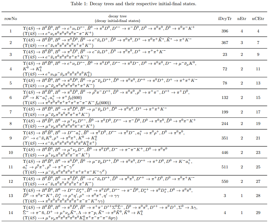
The column headers expressed with abbreviations are explained as follows:
Tip
rowNo— row numberiDcyTr— index of decay treenEtr— number of entriesnCEtr— number of cumulative entries
Note
The values of
iDcyTrare assigned from small to large in the program but listed according to the values ofnEtrfrom large to small in the table. This is the reason why they are not in natural order like the values ofrowNo.Considering \(\pi^0\) has a very large production rate and approximately 99% of it decays to \(\gamma \gamma\), the program is designed to discard the decay \(\pi^0 \to \gamma \gamma\) by default at the early phase of processing the input data. As a result, \(\pi^0 \to \gamma \gamma\) does not show itself in the table.
In the table, iDcyTr is the topology tag for decay trees.
Thus, it is also saved in the TTree object of the output root file.
With the C/C++ interpreter of ROOT, you can check it as follow and see
it at the end of the code block.
Similarly, the right side presents the explanations on the command lines and
the key variables.
[zhouxy@ccw04 test]$ root -l                         // Get into the interpreter
root [0] TFile f("MCGenTopo.root")                   // Open the root file
(TFile &) Name: MCGenTopo.root Title:
root [1] f.ls()                                      // List the objects in the root file
TFile**         MCGenTopo.root
 TFile*         MCGenTopo.root
  KEY: TTree    MCGenTopo;1
root [2] MCGenTopo->Show(0)                          // Show the first entry of the TTree object
======> EVENT:0
 __experiment__  = 0
 __run__         = 0
 __event__       = 1
 __production__  = 0
 __weight__      = 1
 nMCGen          = 59                                // nMCGen is the number of the particles
 MCGenPDG_0      = 300553
 MCGenMothIndex_0 = nan
 MCGenPDG_1      = 511
 MCGenMothIndex_1 = 0
 MCGenPDG_2      = -511                              // MCGenPDG_i is the PDG code
 MCGenMothIndex_2 = 0                                              of the i^th particle

 ...

 MCGenPDG_197    = nan                               // MCGenMothIndex_i is the mother index
 MCGenMothIndex_197 = nan                                                of the i^th particle
 MCGenPDG_198    = nan
 MCGenMothIndex_198 = nan
 MCGenPDG_199    = nan
 MCGenMothIndex_199 = nan
 iDcyTr          = 0                                 // This is the newly added topology tag!
root [3] .q                                          // Quit the interpreter
Tip
The topology tag iDcyTr can be used to pick out the entries of specific
decay trees and then examine the distributions of the other quantities over
the decay trees.
This is an important application of topology analysis.
Exercises#
The example above only introduces the basic usage of TopoAna.
You can refer to the documents we introduce in Section 7.7.9 for
more descriptions of the tool.
At the end of this online textbook, we provide the following six exercises for
you to further explore the usage of TopoAna.
You will benefit a lot when you accomplish these exercises.
To do these exercises (except for the first one), you need to look up the proper
setting items in the quick-start tutorial or the user guide we introduce in
Section 7.7.9, add them to the card file, and re-run the program.
Exercise 1
In the example above, we execute basf2 MCGenTopo.py and topoana.exe
topoana.card in two steps. This is a regular practice and does not take
too much efforts. However, sometimes you may want to execute the two command
lines in one step. Could you figure out a way to do this?
Hint
Use the system function of the os module in your python steering script.
Solution
Revise your python steering script by adding import os to the end of its
preamble and appending os.system('topoana.exe topoana.card') at its end,
and then run the script with basf2.
Below is an example of the revised script.
##########################################################################
# basf2 (Belle II Analysis Software Framework)                           #
# Author: The Belle II Collaboration                                     #
#                                                                        #
# See git log for contributors and copyright holders.                    #
# This file is licensed under LGPL-3.0, see LICENSE.md.                  #
##########################################################################
import basf2
from modularAnalysis import inputMdst
from modularAnalysis import variablesToNtuple
from variables.MCGenTopo import mc_gen_topo
import os  # Newly added statement 1!

mypath = basf2.Path()

# load input ROOT file
inputMdst(basf2.find_file('B02D0pi0_D02pi0pi0.root', 'examples', False), mypath)

# Output the variables to a ntuple
variablesToNtuple('', mc_gen_topo(200), 'MCGenTopo', 'MCGenTopo.root', path=mypath)

# Process the events
basf2.process(mypath)

# Invoke the TopoAna program
os.system('topoana.exe topoana.card')  # Newly added statement 2!
Extension
Could you think of another way to do this? For example, with a shell script?
Exercise 2
Try to examine the top 30 decay branches of \(B^{0}\) and all the decay branches of \(D^{*+}\) in the input sample.
Hint
See Section 3 in the quick-start tutorial for the introduction of the setting item.
See Section 3.3 in the user guide for the description of the setting item.
Solution
Add the following setting item to the card file, re-run the program, and check the changes of the output files.
% Component analysis --- decay branches of particles
{
  B0         B0        30
  D*+        Dsp
}
Extension
See Section 3 in the user guide for the description of other similar setting items.
Exercise 3
Try to identify the decay branches \(B^{0} \rightarrow \pi^{0} \bar{D}^{0}\) and \(\bar{B}^{0} \rightarrow \mu^{-} \bar{\nu}_{\mu} D^{*+}\) in the input sample.
Hint
See Section 4 in the quick-start tutorial for the introduction of the setting item.
See Section 4.4 in the user guide for the description of the setting item.
Solution
Add the following setting item to the card file, re-run the program, and check the changes of the output files.
% Signal identification --- decay branches
{
  B0 --> pi0 anti-D0                    &       B2pi0D0bar
  anti-B0 --> D*+ mu- anti-nu_mu        &       B2munuDsp
}
Extension
See Section 4 in the user guide for the description of other similar setting items.
Exercise 4
In the previous example and the above two exercises, we did not consider charge conjugation, which is an important concept in high energy physics. In this exercise, try to process the charge conjugate particles, decay branches, and decay trees together.
Hint
See Section 5 in the quick-start tutorial for the introduction of the setting item.
See Section 5.2.2 in the user guide for the description of the setting item.
Solution
Add the following setting item to the card file, re-run the program, and check the changes of the output files.
% Process charge conjugate objects together (Two options: Y and N. Default: N)
{
  Y
}
Extension
See Section 5.2 in the user guide for the description of other similar setting items.
Exercise 5
Try to impose some cuts to select events. For example, impose one cut
to select only the events with nMCGen>=20 && nMCGen<=40.
Hint
See Section 5.1.1 in the user guide for the description of the setting item.
Solution
Add the following setting item to the card file, re-run the program, and check the changes of the output files.
% Cut to select entries
{
  nMCGen>=20 && nMCGen<=40
}
Extension
See Section 5.1 in the user guide for the description of other similar setting items.
Exercise 6
Try to remove the input TBranch objects nMCGen, MCGenPDG_i, and
MCGenMothIndex_i (i = 0, 1, 2 ...) from the output root files before
the program terminates.
Hint
See Section 5.3.2 in the user guide for the description of the setting item.
Solution
Add the following setting item to the card file, re-run the program, and check the changes of the output files.
% Remove input tbranches from output root files (Two options: Y and N. Default: N)
{
  Y
}
Extension
See Section 5.3 in the user guide for the description of other similar setting items.
Stuck? We can help!
If you get stuck or have any questions to the online book material, the #starterkit-workshop channel in our chat is full of nice people who will provide fast help.
Refer to Collaborative Tools. for other places to get help if you have specific or detailed questions about your own analysis.
Improving things!
If you know how to do it, we recommend you to report bugs and other requests
with GitLab.
Make sure to use the documentation-training label of the basf2 project.
If you just want to give us feedback, please open a GitLab issue and add the label online_book to it.
Please make sure to be as precise as possible to make it easier for us to fix things! So for example:
typos (where?)
missing bits of information (what?)
bugs (what did you do? what goes wrong?)
too hard exercises (which one?)
etc.
If you are familiar with git and want to create your first merge request for the software, take a look at How to contribute. We’d be happy to have you on the team!
Quick feedback!
Do you want to leave us some feedback? Open a GitLab issue and add the label online_book to it.
Author(s) of this lesson
Xing-Yu Zhou