Graph-based Full Event Interpretation

7.8.6. Graph-based Full Event Interpretation#

Author: J. Cerasoli

The Graph-based Full Event Interpretation (graFEI) is a machine learning tool based on deep Graph Neural Networks (GNNs) to inclusively reconstruct events in Belle II using information on the final state particles only, without any prior assumptions about the structure of the underlying decay chain. GNNs are a particular class of neural networks acting on graphs. Graphs are entities composed of a set of nodes \(V=\{v_{i}\}_{i=1}^N`\) connected by edges \(E = \{e_{v_{i} v_{j}} \equiv e_{ij}\}_{i \neq j}\). You can find a brief description of the model in the documentation of the GraFEIModel class.

See also

The model is described in these proceedings. This work is based on ‘Learning tree structures from leaves for particle decay reconstruction’ by Kahn et al. Please consider citing both papers. Part of the code is adapted from the work of Kahn et al (available here). A detailed description of the model is also available in this Belle II internal note (restricted access).

The network is trained to predict the mass hypotheses of final state particles and the Lowest Common Ancestor (LCA) matrix of the event. Each element of the LCA matrix contains the lowest ancestor common to a pair of final state particles. To avoid the use of a unique identifier for each ancestor, a system of classes is used: 6 for \(\Upsilon (4S)\) resonances, 5 for \(B^{\pm,0}\) mesons, 4 for \({D^{*}_{(s)}}^{\pm, 0}\), 3 for \(D^{\pm,0}\), 2 for \(K_{s}^{0}\), 1 for \(\pi^{0}`\) or \(J/\psi\) and 0 for particles not belonging to the decay tree. This new representation of the LCA is called LCAS matrix, where the S stands for “stage”. An example of decay tree with its corresponding LCAS matrix is:

The model can be trained and evaluated in two modes:

\(\Upsilon (4S)\) reconstruction mode: the model is trained to reconstruct the LCAS matrix of the whole event, i.e. the maximum depth of the LCAS matrix is 6;
\(B\) reconstruction mode: the model is trained to reconstruct single \(B\) decays, i.e. the maximum depth of the LCAS matrix is 5. In this case, when applying the model to some data, a signal-side must be reconstructed first, and the graFEI is used to reconstruct the rest-of-event.

Model training#

The graFEI code is contained in analysis/scripts/grafei.

The model is trained with ROOT ntuples produced with the steering file grafei/scripts/create_training_files.py (you may want to modify this file with your own cuts). The file requires the argument -t to be set to either B+, B0 or Ups for \(B^{+}\), \(B^{0}\) or \(\Upsilon (4S)\) reconstruction respectively. This is the only place where you specify which reconstruction mode you wish to perform: the code will figure it out automatically in later steps. The output files used for training and evaluation must be placed in the folders root/train and root/val respectively, where root is a folder of your choice.

The training is performed with the python script grafei/scripts/train_model.py. It requires a .yaml config file with the -c argument. You can find a prototype of config file at analysis/data/grafei_config.yaml, where all options are documented. The training outputs a copy of the config file used and a weight file in the format .pt that can be used to apply the model to some other data. The output folder is defined in the config file.

Note

Example of running create_training_file.py:

basf2 create_training_file.py -i PATH/TO/SOMENTUPLE.mdst -n 1000 -- -t Ups

Example of running train_model.py:

python3 train_model.py -c PATH/TO/SOMECONFIG.yaml

The loss function is of the form

\[\mathcal{L} = \text{Cross-entropy}_{\text{LCA}} + \alpha \cdot \text{Cross-entropy}_{\text{Masses}},\]

where \(\alpha\) is a parameter tunable in the config file.

Applying the model to data#

The model .yaml and .pt output files can be saved to a payload with the script grafei/scripts/save_model_to_payload.py and uploaded to a global tag in order to run on the grid.

Finally, the model can be included in a steering file via the graFEI wrapper function, in order to apply the model to Belle II data and MC. Example of steering files for \(B\) and \(\Upsilon (4S)\) reconstruction modes are available in analysis/examples/GraFEI. In both cases the LCAS matrix is not directly saved in the final ntuples, but several variables labelled with the prefix graFEI_ are available. When using the model in \(\Upsilon (4S)\) reconstruction mode you have also the possibility of specifying an LCAS matrix (in the form of a nested list) and a list of mass hypotheses (following the convention outlined in the select_good_decay class) for your signal-side: in the case where the predicted LCAS matrix describes a valid tree structure, the code checks if a subset of particles in the tree matches the given LCAS and mass hypotheses (the ordering of the final state particles does not matter because all the permutations are checked, however the mass hypotheses and the LCAS rows/columns should match). If so, the graFEI_goodEvent variable is set to 1. This allows to get rid of badly reconstructed events. If you pass a list of particle lists as input to the model (more information in the graFEI documentation) the mass hypotheses of final state particles are updated to match those predicted by the model and stored in new particle lists called PART:graFEI. In this case you can construct signal- and tag-side candidates with the following lines of code (as documented in the example):

charged_types = ["e+", "mu+", "pi+", "K+", "p+"]
particle_types = charged_types + ["gamma"]

# Define sig-side B -> K+ (nu nu)
ma.reconstructDecay(
   f"B+:sgn -> K+:graFEI",
   "daughter(0, extraInfo(graFEI_sigSide)) == 1",
   path=path,
)

# Define tag-side B
for part in particle_types:
    ma.cutAndCopyList(
       f"{part}:Btag",
       f"{part}:graFEI",
       cut="extraInfo(graFEI_sigSide) == 0",
       writeOut=True,
       path=path,
    )
ma.combineAllParticles([f"{part}:Btag" for part in particle_types], "B+:Btag", path=path)

ma.reconstructDecay("Upsilon(4S):neutral -> B+:Bsgn B-:Btag",
                    "",
                    path=path)
ma.reconstructDecay("Upsilon(4S):charged -> B+:Bsgn B+:Btag",
                    "",
                    allowChargeViolation=True,
                    path=path)

ma.copyLists(
        "Upsilon(4S):graFEI",
        [
            "Upsilon(4S):neutral",
            "Upsilon(4S):charged",
        ],
        path=path,
    )

The extraInfo(graFEI_sigSide) is set to 1 for particles predicted to belong to the signal-side, 0 for particles predicted to belong to the tag-side and -1 for particles in events with graFEI_goodEvent = 0. Therefore, if you want meaningful distributions you should cut on events with graFEI_goodEvent = 1. However, if you reconstruct the signal-side as in the example, only good events are kept.

The variables added by the GraFEI are filled with nan if there are less than two reconstructed particles in the event. Otherwise, they are defined as follows:

Variable	Description
`graFEI_probEdgeProd`	Discriminating variable obtained as the product of predicted edge class probabilities in the event.
`graFEI_probEdgeMean`	Discriminating variable obtained as the arithmetic mean of predicted edge class probabilities in the event.
`graFEI_probEdgeGeom`	Discriminating variable obtained as the geometric mean of predicted edge class probabilities in the event.
`graFEI_validTree`	1 for valid tree structures, 0 otherwise.
`graFEI_goodEvent`	1 for events having a correctly reconstructed signal-side, 0 otherwise (\(\Upsilon (4S)\) reconstruction mode only).
`graFEI_nFSP`	Number of reconstructed final state particles in the event.
`graFEI_nCharged_preFit`	Number of reconstructed charged particles in the event, according to mass hypotheses assigned with likelihood functions.
`graFEI_nPhotons_preFit`	Number of reconstructed photons in the event, according to mass hypotheses assigned with likelihood functions.
`graFEI_nElectrons_preFit`	Number of reconstructed electrons in the event, according to mass hypotheses assigned with likelihood functions.
`graFEI_nMuons_preFit`	Number of reconstructed muons in the event, according to mass hypotheses assigned with likelihood functions.
`graFEI_nPions_preFit`	Number of reconstructed pions in the event, according to mass hypotheses assigned with likelihood functions.
`graFEI_nKaons_preFit`	Number of reconstructed kaons in the event, according to mass hypotheses assigned with likelihood functions.
`graFEI_nProtons_preFit`	Number of reconstructed protons in the event, according to mass hypotheses assigned with likelihood functions.
`graFEI_nLeptons_preFit`	Number of reconstructed leptons in the event, according to mass hypotheses assigned with likelihood functions.
`graFEI_nOthers_preFit`	Number of other reconstructed particles in the event, according to mass hypotheses assigned with likelihood functions.
`graFEI_nCharged_postFit`	Number of reconstructed charged particles in the event, according to mass hypotheses assigned with the graFEI model.
`graFEI_nPhotons_postFit`	Number of reconstructed photons in the event, according to mass hypotheses assigned with the graFEI model.
`graFEI_nElectrons_postFit`	Number of reconstructed electrons in the event, according to mass hypotheses assigned with the graFEI model.
`graFEI_nMuons_postFit`	Number of reconstructed muons in the event, according to mass hypotheses assigned with the graFEI model.
`graFEI_nPions_postFit`	Number of reconstructed pions in the event, according to mass hypotheses assigned with the graFEI model.
`graFEI_nKaons_postFit`	Number of reconstructed kaons in the event, according to mass hypotheses assigned with the graFEI model.
`graFEI_nProtons_postFit`	Number of reconstructed protons in the event, according to mass hypotheses assigned with the graFEI model.
`graFEI_nLeptons_postFit`	Number of reconstructed leptons in the event, according to mass hypotheses assigned with the graFEI model.
`graFEI_nOthers_postFit`	Number of other reconstructed particles in the event, according to mass hypotheses assigned with the graFEI model.
`graFEI_nPredictedUnmatched`	Number of reconstructed particles predicted as being “unmatched” by the model, i.e. the corresponding line in the LCAS matrix is filled with 0’s.
`graFEI_nPredictedUnmatched_noPhotons`	Number of reconstructed particles predicted as being “unmatched” by the model, excluding photons.
`graFEI_truth_perfectLCA`	Truth-matching variable: 1 if LCAS matrix of the event if perfectly reconstructed, 0 otherwise.
`graFEI_truth_perfectMasses`	Truth-matching variable: 1 if all mass hypotheses in the event are perfectly assigned, 0 otherwise.
`graFEI_truth_perfectEvent`	Truth-matching variable: logical `AND` of `perfectLCA` and `perfectMasses`.
`graFEI_truth_isSemileptonic`	Truth-matching variable: 1 if a neutrino is present in the true underlying decay chain, 0 if not present, -1 if no decay chain can be matched to the event.
`graFEI_truth_nFSP`	Truth-matching variable: number of final state particles in the true underlying decay chain, -1 if no decay chain can be matched to the event.
`graFEI_truth_nPhotons`	Truth-matching variable: number of final state particles matched to true photons.
`graFEI_truth_nElectrons`	Truth-matching variable: number of final state particles matched to true electrons.
`graFEI_truth_nMuons`	Truth-matching variable: number of final state particles matched to true muons.
`graFEI_truth_nPions`	Truth-matching variable: number of final state particles matched to true pions.
`graFEI_truth_nKaons`	Truth-matching variable: number of final state particles matched to true kaons.
`graFEI_truth_nProtons`	Truth-matching variable: number of final state particles matched to true protons.
`graFEI_truth_nOthers`	Truth-matching variable: number of final state particles matched to true other particles.

Code documentation#

This section describes the grafei code.

Core modules#

If you want to use a custom steering file to create training data, you can import the LCASaverModule with from grafei import lcaSaver. You can import the core GraFEIModule in a steering file with from grafei import graFEI. These are wrapper functions that internally call the modules and add them to the basf2 path.

grafei.graFEI(list_name, path, particle_lists=None, store_mc_truth=False, cfg_path=None, param_file=None, sig_side_lcas=None, sig_side_masses=None, gpu=False, payload_config_name='graFEIConfigFile', payload_model_name='graFEIModelFile')[source]#

Wrapper function to add the GraFEIModule to the path and perform other actions behind the scenes.

Applies graFEI model to a (list of) particle list(s) in basf2. GraFEI information is stored as eventExtraInfos.

Note

list_name should always be provided. This is the name of the particle list to be given as input to the graFEI. If list_name refers to an existing particle list, it is used as input to the model. If also a list of final state particle lists is provided in particle_lists, these are combined to form a new list called list_name (if list_name already exists an error is thrown). If particle_list is provided, the mass hypotheses of final state particles are updated to match graFEI predictions.

Parameters:

list_name (str) – Name of particle list given as input to the model.
path (basf2.Path) – Module is added to this path.
particle_lists (list) – List of particle lists. If provided, these are combined to form list_name.
store_mc_truth (bool) – Whether to store MC truth information.
cfg_path (str) – Path to config file. If None the config file in the global tag is used.
param_file (str) – Path to parameter file containing the model. If None the parameter file in the global tag is used.
sig_side_lcas (list) – List containing LCAS matrix of signal-side.
sig_side_masses (list) – List containing mass hypotheses of signal-side.
gpu (bool) – Whether to run on a GPU.
payload_config_name (str) – Name of config file payload. The default should be kept, except in basf2 examples.
payload_model_name (str) – Name of model file payload. The default should be kept, except in basf2 examples.

Returns:

List of graFEI variables.

Return type:

list

grafei.lcaSaver(particle_lists, features, mcparticle_list, output_file, path)[source]#

Wrapper function to add the LCASaverModule to the path.

Save Lowest Common Ancestor matrix of each MC Particle in the given list.

Parameters:

particle_lists (list) – Name of particle lists to save features of.
features (list) – List of features to save for each particle.
mcparticle_list (str) – Name of particle list to build LCAs from (used as root).
output_file (str) – Path to output file to save.
path (basf2.Path) – Module is added to this path.

Other modules and functions#

Here the core code of the graFEI is described. This section is intended for developers, users usually do not need to manipulate these components.

grafei.model.config.load_config(cfg_path=None, model=None, dataset=None, run_name=None, samples=None, **kwargs)[source]#

Load default configs followed by user configs and populate dataset tags.

Parameters:

cfg_path (str or Path) – Path to user config yaml.
model (str) – Name of model to use (overwrites loaded config).
dataset (int) – Individual dataset to load (overwrites loaded config).
run_name (str) – Name of training run (overwrites loaded config).
samples (int) – Number of samples to train on (overwrites loaded config).

Returns:

Loaded training configuration dictionary and list of tuples containing (tag name, dataset path, tag key).

Return type:

dict, list

class grafei.model.create_trainer.GraFEIIgniteTrainer(model, optimizer, loss_fn, device, configs, tags, scheduler=None, ignore_index=-1.0)[source]#

Class to setup the ignite trainer and hold all the things associated.

Parameters:

model (Model) – The actual PyTorch model.
optimizer (Optimizer) – Optimizer used in training.
loss_fn (Loss) – Loss function.
device (Device) – Device to use.
configs (dict) – Dictionary of run configs from loaded yaml config file.
tags (list) – Various tags to sort train and validation evaluators by, e.g. “Training”, “Validation”.
scheduler (Scheduler) – Learning rate scheduler.
ignore_index (int) – Label index to ignore when calculating metrics, e.g. padding.

grafei.model.dataset_split.create_dataloader_mode_tags(configs, tags)[source]#

Convenience function to create the dataset/dataloader for each mode tag (train/val) and return them.

Parameters:

configs (dict) – Training configuration.
tags (list) – Mode tags train/val containing dataset paths.

Returns:

Mode tag dictionary containing tuples of (mode, dataset, dataloader).

Return type:

dict

grafei.model.dataset_utils.populate_avail_samples(X, Y, B_reco=0)[source]#

Shifts through the file metadata to populate a list of available dataset samples.

Parameters:

X (list) – List of ROOT lazyarray dicts for X (input) data.
Y (list) – List of ROOT lazyarray dicts for Y (ground truth) data.
B_reco (int) –
Reconstruction mode flag (set automatically):

\[\text{Upsilon} (4S) = 0,\ B^0 = 1,\ B^+ = 2.\]

Returns:

List of available samples for training.

Return type:

list

grafei.model.dataset_utils.preload_root_data(root_files, features, discarded)[source]#

Load all data from root files as lazyarrays (not actually read from disk until accessed).

Parameters:

root_files (str) – Path to ROOT files.
features (list) – List of feature names.
discarded (list) – List of features present in the ROOT files and not used as input, but used to calculate other quantities (e.g. edge features).

Returns:

Lists of dictionaries containing training information for input and ground-truth.

Return type:

list, list

grafei.model.edge_features.compute_cosTheta(name_values)[source]#

Computes cosinus of angle between two tracks.

Parameters:: name_values (dict) – Dictionary of numpy arrays containing p, px, py, pz.
Returns:: Array containing cosinus of theta values.
Return type:: numpy.ndarray

grafei.model.edge_features.compute_doca(name_values)[source]#

Computes DOCA between two tracks.

Parameters:: name_values (dict) – Dictionary of numpy arrays containing px, py, pz, x, y, z.
Returns:: Array containing doca values.
Return type:: numpy.ndarray

grafei.model.edge_features.compute_edge_features(edge_feature_names, features, x)[source]#

Computes a series of edge features starting from node features.

Parameters:

edge_feature_names (list) – List of edge features names.
features (list) – List of node feature names.
x (numpy.ndarray) – Array of node features.

Returns:

Array of edge features.

Return type:

numpy.ndarray

class grafei.model.geometric_datasets.GraphDataSet(root, n_files=None, samples=None, features=[], edge_features=[], global_features=[], normalize=None, **kwargs)[source]#

Dataset handler for converting Belle II data to PyTorch geometric InMemoryDataset.

The ROOT format expects the tree in every file to be named Tree, and all node features to have the format feat_FEATNAME.

Note

This expects the files under root to have the structure root/**/<file_name>.root where the root path is different for train and val. The **/ is to handle subdirectories, e.g. sub00.

Parameters:

root (str) – Path to ROOT files.
n_files (int) – Load only n_files files.
samples (int) – Load only samples events.
features (list) – List of node features names.
edge_features (list) – List of edge features names.
global_features (list) – List of global features names.
normalize (bool) – Whether to normalize input features.

class grafei.model.geometric_layers.EdgeLayer(nfeat_in_dim, efeat_in_dim, gfeat_in_dim, efeat_hid_dim, efeat_out_dim, num_hid_layers, dropout, normalize=True)[source]#

Updates edge features in MetaLayer:

\[e_{ij}^{'} = \phi^{e}(e_{ij}, v_{i}, v_{j}, u),\]

where \(\phi^{e}\) is a neural network of the form

Parameters:

nfeat_in_dim (int) – Node features input dimension (number of node features in input).
efeat_in_dim (int) – Edge features input dimension (number of edge features in input).
gfeat_in_dim (int) – Global features input dimension (number of global features in input).
efeat_hid_dim (int) – Edge features dimension in hidden layers.
efeat_out_dim (int) – Edge features output dimension.
num_hid_layers (int) – Number of hidden layers.
dropout (float) – Dropout rate \(r \in [0,1]\).
normalize (str) – Type of normalization (batch/layer).

Returns:

Updated edge features tensor.

Return type:

Tensor

class grafei.model.geometric_layers.GlobalLayer(nfeat_in_dim, efeat_in_dim, gfeat_in_dim, gfeat_hid_dim, gfeat_out_dim, num_hid_layers, dropout, normalize=True)[source]#

Updates node features in MetaLayer:

\[u_{i}^{'} = \phi^{u}(\rho^{e \to u}(e), \rho^{v \to u}(v), u)\]

with

\[\begin{split}\rho^{e \to u}(e) = \frac{\sum_{i,j=1,\ i \neq j}^{N} e_{ij}}{N \cdot (N-1)},\\ \rho^{v \to u}(e) = \frac{\sum_{i=1}^{N} v_{i}}{N},\end{split}\]

where \(\phi^{u}\) is a neural network of the form

Parameters:

nfeat_in_dim (int) – Node features input dimension (number of node features in input).
efeat_in_dim (int) – Edge features input dimension (number of edge features in input).
gfeat_in_dim (int) – Global features input dimension (number of global features in input).
nfeat_hid_dim (int) – Global features dimension in hidden layers.
nfeat_out_dim (int) – Global features output dimension.
num_hid_layers (int) – Number of hidden layers.
dropout (float) – Dropout rate \(r \in [0,1]\).
normalize (str) – Type of normalization (batch/layer).

Returns:

Updated global features tensor.

Return type:

Tensor

class grafei.model.geometric_layers.NodeLayer(nfeat_in_dim, efeat_in_dim, gfeat_in_dim, nfeat_hid_dim, nfeat_out_dim, num_hid_layers, dropout, normalize=True)[source]#

Updates node features in MetaLayer:

\[v_{i}^{'} = \phi^{v}(v_{i}, \rho^{e \to v}(v_{i}), u)\]

with

\[\rho^{e \to v}(v_{i}) = \frac{\sum_{j=1,\ j \neq i}^{N} (e_{ji} + e _{ij})}{2 \cdot (N-1)},\]

where \(\phi^{v}\) is a neural network of the form

Parameters:

nfeat_in_dim (int) – Node features input dimension (number of node features in input).
efeat_in_dim (int) – Edge features input dimension (number of edge features in input).
gfeat_in_dim (int) – Global features input dimension (number of global features in input).
nfeat_hid_dim (int) – Node features dimension in hidden layers.
nfeat_out_dim (int) – Node features output dimension.
num_hid_layers (int) – Number of hidden layers.
dropout (float) – Dropout rate \(r \in [0,1]\).
normalize (str) – Type of normalization (batch/layer).

Returns:

Updated node features tensor.

Return type:

Tensor

class grafei.model.geometric_network.GraFEIModel(nfeat_in_dim, efeat_in_dim, gfeat_in_dim, edge_classes=6, x_classes=7, hidden_layer_dim=128, num_hid_layers=1, num_ML=1, dropout=0.0, global_layer=True, **kwargs)[source]#

Actual implementation of the model, based on the MetaLayer class.

The network is composed of:

A first MetaLayer to increase the number of nodes and edges features;
A number of intermediate MetaLayers (tunable in config file);
A last MetaLayer to decrease the number of node and edge features to the desired output dimension.

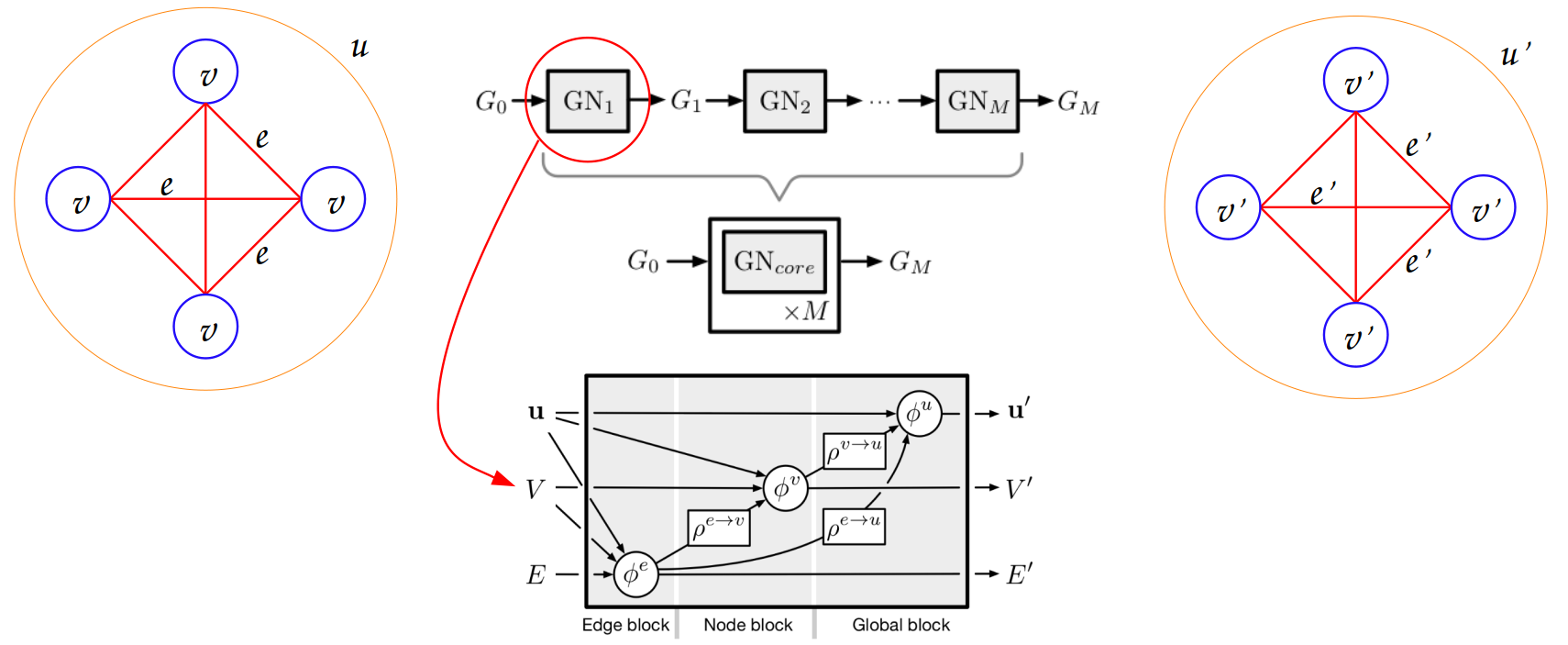
Each MetaLayer is in turn composed of EdgeLayer, NodeLayer and GlobalLayer sub-blocks.

Parameters:

nfeat_in_dim (int) – Node features dimension (number of input node features).
efeat_in_dim (int) – Edge features dimension (number of input edge features).
gfeat_in_dim (int) – Global features dimension (number of input global features).
edge_classes (int) – Edge features output dimension (i.e. number of different edge labels in the LCAS matrix).
x_classes (int) – Node features output dimension (i.e. number of different mass hypotheses).
hidden_layer_dim (int) – Intermediate features dimension (same for node, edge and global).
num_hid_layers (int) – Number of hidden layers in every MetaLayer.
num_ML (int) – Number of intermediate MetaLayers.
dropout (float) – Dropout rate \(r \in [0,1]\).
global_layer (bool) – Whether to use global layer.

Returns:

Node, edge and global features after model evaluation.

Return type:

tuple(Tensor)

exception grafei.model.lca_to_adjacency.InvalidLCAMatrix[source]#: Specialized Exception sub-class raised for malformed LCA matrices or LCA matrices not encoding trees.

class grafei.model.lca_to_adjacency.Node(level, children, lca_index=None, lcas_level=0)[source]#

Class to hold levels of nodes in the tree.

Parameters:

level (int) – Level in the tree.
children (list[Node]) – Children of the nodes.
lca_index (int) – Index in the LCAS matrix.
lcas_level (int) – Level in the LCAS matrix.

grafei.model.lca_to_adjacency.lca_to_adjacency(lca_matrix)[source]#

Converts a tree’s LCA matrix representation, i.e. a square matrix (M, M) where each row/column corresponds to a leaf of the tree and each matrix entry is the level of the lowest-common-ancestor (LCA) of the two leaves, into the corresponding two-dimension adjacency matrix (N,N), with M < N. The levels are enumerated top-down from the root.

See also

The pseudocode for LCA to tree conversion is described in Kahn et al.

Parameters:

lca_matrix – 2-dimensional LCA matrix (M, M).

Returns:

2-dimensional matrix (N, N) encoding the graph’s node adjacencies. Linked nodes have values unequal to zero.

Return type:

Tensor

Raises:

InvalidLCAMatrix – If passed LCA matrix is malformed (e.g. not 2d or not square) or does not encode a tree.

grafei.model.lca_to_adjacency.select_good_decay(predicted_lcas, predicted_masses, sig_side_lcas=None, sig_side_masses=None)[source]#

Checks if given LCAS matrix is found in reconstructed LCAS matrix and mass hypotheses are correct.

Warning

You have to make sure to call this function only for valid tree structures encoded in predicted_lcas, otherwise it will throw an exception.

Mass hypotheses are indicated by letters. The following convention is used:

\[\begin{split}'e' \to e \\ 'i' \to \pi \\ 'k' \to K \\ 'p' \to p \\ 'm' \to \mu \\ 'g' \to \gamma \\ 'o' \to \text{others}\end{split}\]

Warning

The order of mass hypotheses should match that of the final state particles in the LCAS.

Parameters:

predicted_lcas – LCAS matrix.
predicted_masses (list[str]) – List of predicted mass classes.
sig_side_lcas – LCAS matrix of your signal-side.
sig_side_masses (list[str]) – List of mass hypotheses for your FSPs.

Returns:

True if LCAS and masses match, LCAS level of root node, LCA indices of FSPs belonging to the signal side ([-1] if LCAS does not match decay string).

Return type:

bool, int, list

class grafei.model.metrics.PerfectEvent(ignore_index, output_transform, device='cpu')[source]#

Computes the rate of events with perfectly predicted mass hypotheses and LCAS matrices over a batch.

output_transform should return the following items: (x_pred, x_y, edge_pred, edge_y, edge_index, u_y, batch, num_graphs).

x_pred must contain node prediction logits and have shape (num_nodes_in_batch, node_classes);
x_y must contain node ground-truth class indices and have shape (num_nodes_in_batch, 1);
edge_pred must contain edge prediction logits and have shape (num_edges_in_batch, edge_classes);
edge_y must contain edge ground-truth class indices and have shape (num_edges_in_batch, 1);
edge index maps edges to its nodes;
u_y is the signal/background class (always 1 in the current setting);
batch maps nodes to their graph;
num_graphs is the number of graph in a batch (could be derived from batch also).

See also

Ignite metrics

Parameters:

ignore_index (list[int]) – Class or list of classes to ignore during the computation (e.g. padding).
output_transform (function) – Function to transform engine’s output to desired output.
device (str) – cpu or gpu.

class grafei.model.metrics.PerfectLCA(ignore_index, output_transform, device='cpu')[source]#

Computes the rate of perfectly predicted LCAS matrices over a batch.

output_transform should return the following items: (edge_pred, edge_y, edge_index, u_y, batch, num_graphs).

edge_pred must contain edge prediction logits and have shape (num_edges_in_batch, edge_classes);
edge_y must contain edge ground-truth class indices and have shape (num_edges_in_batch, 1);
edge index maps edges to its nodes;
u_y is the signal/background class (always 1 in the current setting);
batch maps nodes to their graph;
num_graphs is the number of graph in a batch (could be derived from batch also).

See also

Ignite metrics

Parameters:

ignore_index (list[int]) – Class or list of classes to ignore during the computation (e.g. padding).
output_transform – Function to transform engine’s output to desired output.
device (str) – cpu or gpu.

class grafei.model.metrics.PerfectMasses(ignore_index, output_transform, device='cpu')[source]#

Computes the rate of events with perfectly predicted mass hypotheses over a batch.

output_transform should return the following items: (x_pred, x_y, u_y, batch, num_graphs).

x_pred must contain node prediction logits and have shape (num_nodes_in_batch, node_classes);
x_y must contain node ground-truth class indices and have shape (num_nodes_in_batch, 1);
u_y is the signal/background class (always 1 in the current setting);
batch maps nodes to their graph;
num_graphs is the number of graph in a batch (could be derived from batch also).

See also

Ignite metrics

Parameters:

ignore_index (list[int]) – Class or list of classes to ignore during the computation (e.g. padding).
output_transform – Function to transform engine’s output to desired output.
device (str) – cpu or gpu.

class grafei.model.multiTrain.MultiTrainLoss(alpha_mass=0, ignore_index=-1, reduction='mean')[source]#

Sum of cross-entropies for training against LCAS and mass hypotheses.

Parameters:

alpha_mass (float) – Weight of mass cross-entropy term in the loss.
ignore_index (int) – Index to ignore in the computation (e.g. padding).
reduction (str) – Type of reduction to be applied on the batch (sum or mean).

grafei.model.normalize_features.normalize_features(normalize={}, features=[], x=[], edge_features=[], x_edges=[], global_features=[], x_global=[])[source]#

Function to normalize input features.

normalize should be a dictionary of the form {'power', [0.5], 'linear', [-0.5, 4.1]}. power and linear are the only processes supported.

Parameters:

normalize (dict) – Normalization processes and parameters.
features (list) – List of node feature names.
x (numpy.ndarray) – Array of node features.
edge_features (list) – List of edge feature names.
x_edges (numpy.ndarray) – Array of edge features.
global_features (list) – List of global feature names.
x_global (numpy.ndarray) – Array of global features.

grafei.model.tree_utils.is_valid_tree(adjacency_matrix)[source]#

Checks whether the graph encoded by the passed adjacency matrix encodes a valid tree, i.e. an undirected, acyclic and connected graph.

Parameters:: adjacency_matrix (numpy.ndarray) – 2-dimensional matrix (N, N) encoding the graph’s node adjacencies. Linked nodes should have value unequal to zero.
Returns:: True if the encoded graph is a tree, False otherwise.
Return type:: bool

grafei.model.tree_utils.masses_to_classes(array)[source]#

Converts mass hypotheses to classes used in cross-entropy computation.

Classes are:

\[\begin{split}e \to 1\\ \mu \to 2\\ \pi \to 3\\ K \to 4\\ p \to 5\\ \gamma \to 6\\ \text{others} \to 0\end{split}\]

Parameters:: array (numpy.ndarray) – Array containing PDG mass codes.
Returns:: Array containing mass hypothese converted to classes.
Return type:: numpy.ndarray

class grafei.modules.LCASaverModule.LCASaverModule(particle_lists, features, mcparticle_list, output_file)[source]#

Save Lowest Common Ancestor matrix of each MC Particle in the given list.

Parameters:

particle_lists (list) – Name of particle lists to save features of.
features (list) – List of features to save for each particle.
mcparticle_list (str) – Name of particle list to build LCAs from (will use as root).
output_file (str) – Path to output file to save.

grafei.modules.LCASaverModule.get_object_list(pointerVec)[source]#

Workaround to avoid memory problems in basf2.

Parameters:: pointerVec – Input particle list.
Returns:: Output python list.
Return type:: list

grafei.modules.LCASaverModule.pdg_to_lca_converter(pdg)[source]#

Converts PDG code to LCAS classes.

Tip

If you want to modify the LCAS classes, it’s here. Don’t forget to update the number of edge classes accordingly in the yaml file.

Parameters:: pdg (int) – PDG code to convert.
Returns:: Corresponding LCAS class, or None if PDG not present in pdg_lca_match.
Return type:: int or None

grafei.modules.LCASaverModule.write_hist(particle, leaf_hist={}, levels={}, hist=[], pdg={}, leaf_pdg={}, semilep_flag=False)[source]#

Recursive function to traverse down to the leaves saving the history.

Parameters:: particle – The current particle being inspected. Other arguments are automatically set.

class grafei.modules.GraFEIModule.GraFEIModule(particle_list, cfg_path=None, param_file=None, sig_side_lcas=None, sig_side_masses=None, gpu=False, payload_config_name='graFEIConfigFile', payload_model_name='graFEIModelFile')[source]#

Applies graFEI model to a particle list in basf2. GraFEI information is stored as extraInfos.

Parameters:

particle_list (str) – Name of particle list.
cfg_path (str) – Path to config file. If None the config file in the global tag is used.
param_file (str) – Path to parameter file containing the model. If None the parameter file in the global tag is used.
sig_side_lcas (list) – List containing LCAS matrix of signal-side.
sig_side_masses (list) – List containing mass hypotheses of signal-side.
gpu (bool) – Whether to run on a GPU.
payload_config_name (str) – Name of config file payload. The default should be kept, except in basf2 examples.
payload_model_name (str) – Name of model file payload. The default should be kept, except in basf2 examples.

Graph-based Full Event Interpretation

Contents

7.8.6. Graph-based Full Event Interpretation#

Model training#

Applying the model to data#

Code documentation#

Core modules#

Other modules and functions#