3.4.10. Continuum Suppression (CS)#

Introduction#

Most e⁺ e^- interactions at Belle II do not result in a ϒ(4S) resonance which then decays to two B mesons.

Of these non-ϒ(4S) events, those resulting in some state without hadrons are usually not problematic in analyses looking for B decays as they are already rejected by the trigger.

Continuum events are more problematic. B meson candidates reconstructed from these decays show a broad distribution in variables such as the beam-constrained mass which makes them difficult to separate and suppress when extracting a signal component.

Question

Do you still remember what continuum is?

Hint

Have a look back in Backgrounds, backgrounds, backgrounds where this is introduced.

Solution

When we talk about continuum, we mean events with the process e⁺ e^- → qq, i.e. directly to some lighter hadrons without creating a ϒ(4S) resonance.

In Belle II Monte Carlo, the centrally produced continuum samples are separated by their quark content and are called uubar, ddbar, ssbar, and ccbar.

If variables which you already know from the previous exercises are bad at separating continuum and BB events, which other properties of the events can we use? The answer is the overall shape of the events, i.e. the momentum-weighted distribution of all particles in the detector.

Question

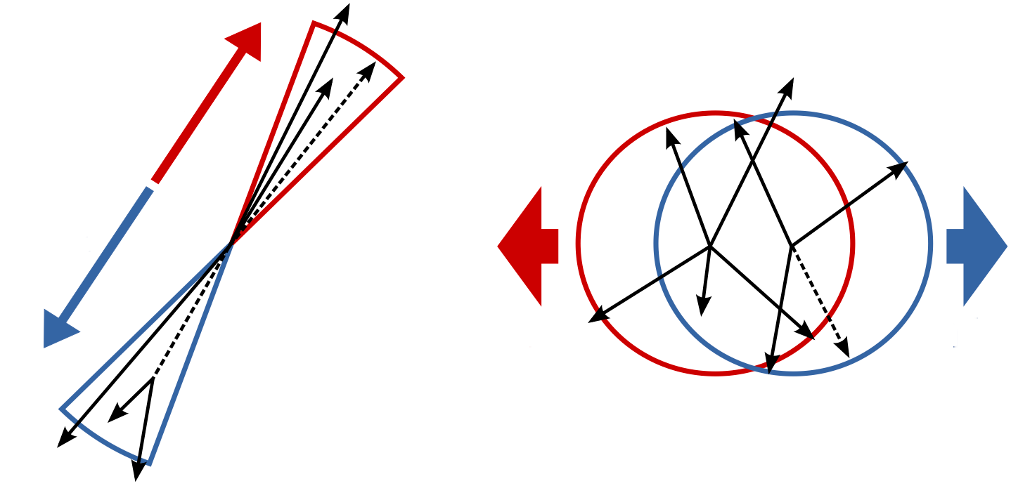
Which of these two pictures better represents the distribution (shape) of particles you would expect in a BB event? Which represents a continuum event?

../../_images/continuum_without_labels.png

Hint

Think about the different masses of the Continuum hadrons compared to B mesons. How does this reflect in the momentum?

Solution

The continuum particles are strongly collimated due to the large available momentum for the decay to light hadrons. In contrast, the particles from the BB event are uniformly distributed.

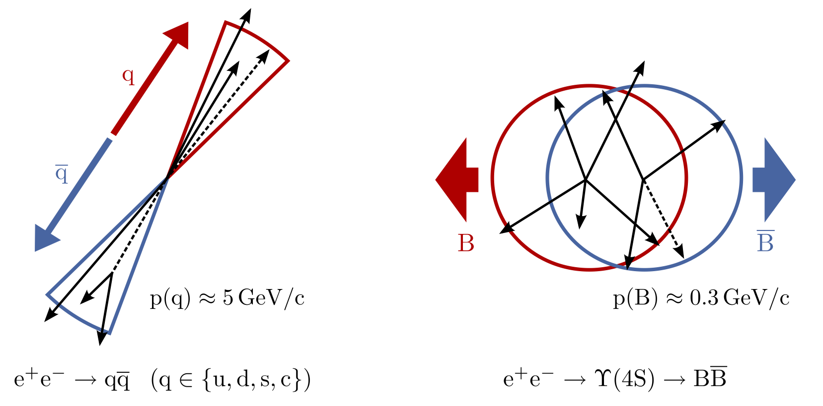
../../_images/continuum_with_labels.png — Fig. 3.28 (Credit: Markus Röhrken)#

So how do we get access to the event shape? We construct B candidates and then create a Rest of Event for them. This allows us to study the entire event and compute shape properties, while taking into account which particles belong to our signal reconstruction.

Warning

In addition to the Continuum suppression tools that we will be using in this exercise, there is also the EventShape framework in basf2 which calculates similar properties to the Continuum Suppression module. However, this does not use candidate-based analysis and is not designed for Continuum Suppression.

Always make sure the variables you’re using in the exercise are from the Continuum Suppression module and not the similarly-named ones from the Event Shape Framework.

Which properties can we use? A popular one is the ratio of the second and zeroth Fox-Wolfram moment:

\[R_2 = \frac{H_2}{H_0}\]

This variable is called R2 in basf2 (not to be confused with foxWolframR2 which is the same property but from the Event Shape Framework).

Fox-Wolfram moments are rotationally-invariant parametrisations of the distribution of particles in an event. They are defined by

\[H_l = \sum_{i,j} \frac{\lvert p_i \rvert \lvert p_j \rvert }{E^2_{\text{event}}} P_l(\cos{\theta_{i, j}})\]

with the momenta p _i,j, the angle θ _i,j between them, the total energy in the event E _event and the Legendre Polynomials P _l.

Other powerful properties are those based on the thrust vector. This is the vector along which the total projection of a collection of momenta is maximised. This collection of momenta can be the B candidate or the rest of event.

The cosine of the angle between both thrust vectors, cosTBTO in basf2, is a thrust-based discriminating variable. In BB events, the particles are almost at rest and so the thrust vectors are uniformly distributed. Therefore, cosTBTO will also be uniformly distributed between 0 and 1. In qq events, the particles are collimated and the thrust axes point back-to-back, leading to a peak at high values of cosTBTO. A similar argument can be made for the angle of the thrust axis with the beam axis which is cosTBz in basf2.

In addition to the angular quantities, basf2 also provides the total thrust magnitude of both the B candidate thrustBm and the ROE thrustOm. Depending on the signal process, these can also provide some discriminating power.

If you would like to know more, Chapter 9 of The Physics of the B Factories book has an extensive overview over these quantities.

Question

Can you find out which other variables are provided by basf2 for continuum suppression?

Hint

Check the Continuum Suppression variable group in Variables.

Solution

In addition to the five variables

mentioned above, basf2 also provides “CLEO cones” (CleoConeCS) and “Kakuno-Super-Fox-Wolfram” variables (KSFWVariables). These are more complex engineered variables and are mostly used with machine learning methods.

First Continuum Suppression steps in basf2#

Now, how do we access the shape of events in basf2?

First we need some data. In this exercise we will use two samples, one with “uubar” continuum background and one with \(B^0 \to K_S^0 \pi^0\) decays. These samples are called uubar_sample.root and B02ks0pi0_sample.root and can be used with the basf2.find_file function (you need the data_type='examples' switch and also have to prepend starterkit/2021/ to the filename). If this doesn’t work you can find the files in /sw/belle2/examples-data/starterkit/2021 on KEKCC.

Exercise

Load the mdst files mentioned above, then reconstruct Kshort candidates from two charged pions. Load the charged pions with the cut 'chiProb > 0.001 and pionID > 0.5' and combine only pions whose combined invariant mass is within 36 MeV of the neutral kaon mass (498 MeV). We won’t be using the Kshorts from the stdV0s package as these are always vertex fit which we don’t need.

Then, load some neutral pion candidates from stdPi0s and combine them with the Kshort candidates to B0 candidates. Only create B0 candidates with Mbc between 5.1 GeV and 5.3 GeV and deltaE between -2 GeV and 2 GeV.

These cuts are quite loose but this way you will be able to reconstruct B0 candidates from continuum events without processing large amounts of continuum Monte Carlo.

Solution

#!/usr/bin/env python3

import basf2 as b2
import modularAnalysis as ma
import stdPi0s

# Perform analysis.
main = b2.create_path()

ma.inputMdstList(
    filelist=[
        b2.find_file(
            "starterkit/2021/B02ks0pi0_sample.root", data_type="examples"
        ),
        b2.find_file("starterkit/2021/uubar_sample.root", data_type="examples"),
    ],
    path=main,
)

stdPi0s.stdPi0s(path=main, listtype="eff60_May2020")
ma.fillParticleList(
    decayString="pi+:good", cut="chiProb > 0.001 and pionID > 0.5", path=main
)

ma.reconstructDecay(
    decayString="K_S0 -> pi+:good pi-:good", cut="0.480<=M<=0.516", path=main
)

ma.reconstructDecay(
    decayString="B0  -> K_S0 pi0:eff60_May2020",
    cut="5.1 < Mbc < 5.3 and abs(deltaE) < 2",
    path=main,
)  # [E13]

Exercise

Now, create a Rest of Event for the B0 candidates and append a mask with the track cuts 'nCDCHits > 0 and useCMSFrame(p)<=3.2' and the cluster cuts 'p >= 0.05 and useCMSFrame(p)<=3.2' to it. These cuts are common choices for continuum suppression, however they might not be the best ones for your analysis later on!

Then, adding the continuum suppression module is just a single call to the modularAnalysis.buildContinuumSuppression function. You have to pass the name of the ROE mask you’ve just created to the function.

Hint

You can use modularAnalysis.appendROEMasks to add the mask.

Solution

ma.buildRestOfEvent(target_list_name="B0", path=main)  # [S10]
cleanMask = (
    "cleanMask",
    "nCDCHits > 0 and useCMSFrame(p)<=3.2",
    "p >= 0.05 and useCMSFrame(p)<=3.2",
)
ma.appendROEMasks(list_name="B0", mask_tuples=[cleanMask], path=main)

ma.buildContinuumSuppression(list_name="B0", roe_mask="cleanMask", path=main)  # [E10]

Exercise

Now you can write out a few event shape properties. Use the five properties mentioned above. To evaluate the performance of these variables, add the truth-variable isContinuumEvent.

You can also add the beam-constrained mass Mbc which you should know from previous exercises to see the uniform background component in this variable.

Then, process the path and run the steering file!

Solution

simpleCSVariables = [  # [S20]
    "R2",
    "thrustBm",
    "thrustOm",
    "cosTBTO",
    "cosTBz",
]

ma.variablesToNtuple(
    decayString="B0",
    variables=simpleCSVariables + ["Mbc", "isContinuumEvent"],
    filename="ContinuumSuppression.root",
    treename="tree",
    path=main,
)

b2.process(main)  # [E20]

Now that we have created our ntuple, we can look at the data and see how well the variables suppress continuum.

Exercise

Plot the distributions of R2 from 0 to 1 for both continuum and signal components as determined by isContinuumEvent.

Where would you put the cut when trying to retain as much signal as possible?

If you want you can also plot the other four variables and see how their performance compares.

Hint

Use histtype='step' when plotting with matplotlib, this makes it easier to see the difference between the two distributions.

Solution

# Include this only if running in a Jupyter notebook
# %matplotlib inline

import matplotlib.pyplot as plt
import uproot

var_list = ['isContinuumEvent', 'R2']
df = uproot.open("ContinuumSuppression_applied.root:tree").arrays(var_list, library='pd')

fig, ax = plt.subplots()

signal_df = df.query("(isContinuumEvent == 0.0)")
continuum_df = df.query("(isContinuumEvent == 1.0)")

hist_kwargs = dict(bins=30, range=(0, 1), histtype="step")
ax.hist(signal_df["R2"], label="Not Continuum", **hist_kwargs)
ax.hist(continuum_df["R2"], label="Continuum", **hist_kwargs)
ax.set_xlabel("R2")
ax.set_ylabel("Total number of candidates")
ax.legend()
fig.savefig("R2.pdf")

Your plot should look similar to this:

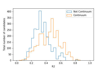
Judging by this plot, a cut at R2 = 0.4 would provide good separation. Of course, this can change if you employ cuts on other CS variables too!

Exercise

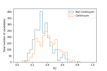
In the previous exercise we have used a uubar sample as our continuum sample. How would you expect the distribution in R2 to change when we switch this out with a ccbar sample? Think about this for a bit, then try it! You can use the file ccbar_sample.root in the starterkit folder.

Solution

The separation becomes worse as the charmed hadrons are heavier and have less momentum:

So how do we separate our signal component from continuum background in the presence of all types of continuum? As you have seen with the five variables we have introduced so far, none of them can provide perfect separation. Fortunately, there is a solution to this: Boosted Decision Trees!

Continuum suppression using Boosted Decision Trees#

Boosted Decision Trees (BDTs) are a specific type of a machine learning model used for classification tasks. In this lesson we try to classify all candidates as either continuum or not continuum.

The name decision tree refers to the general structure: the classification is done with a series of “decisions”. Decisions are logical operations (like “>”, “<”, “=”, etc.) on the input variables of each data point, by the outcome of which the data points are separated into groups. Each outcome has a separate line of decisions following it. The maximum number of such decisions is called the “tree depth”.

The word boosted refers to the specific way the tree is formed: gradient boosting. Gradient boosting means, that a final tree is made by combining a series of smaller trees of a fixed depth.

See also

The reader is welcome to consult the Wikipedia pages on Decision Tree Learning and Gradient Tree Boosting for a more detailed overview. For details on FastBDT, the implementation used at at Belle II take a look at this article. The source code can be found here.

The output of the BDT is the “continuum probability” – the probability of an event being a continuum event, as estimated based on the input variables. The input variables can be in principle any variable that looks different between continuum and non-continuum events. The recommended and most commonly used variables are the ones introduced in the previous lesson as well as others from the Continuum Suppression variable group in the Variables.

The BDT is a supervised machine learning method, i.e. it needs to be trained on a dataset where we know the true class that we are trying to predict (this variable is called the target variable). Thus the steps are

Create a learning dataset (Monte Carlo data)
Make the algorithm “learn” and output a decision tree that we can use.
Apply the trained decision tree to both Monte Carlo and real data.

In the last step, the BDT will return the continuum probability, which then can be stored in the Ntuples. To actually remove continuum events, simply add a cut on the continuum probability at the end.

Exercise

In the three initial exercises of this chapter you’ve learned how to create Ntuples for continuum suppression. We only need some more variables this time.

Create the dataset following the procedure from previous exercises, but also include KSFW moments and CLEO cones into the Ntuples.

Use only the first half of the events for creating these Ntuples.

Hint

Use the code from the previous exercises. Add the new variables to the simpleCSVariables list. See the documentation on the variables in Continuum suppression.

Hint

The files uubar_sample.root and B02ks0pi0_sample.root consist of 2000 and 30000 events respectively. You can choose half for each by using the entrySequences option in the inputMdstList function. See the documentation at ModularAnalysis.

Solution

#!/usr/bin/env python3
import basf2 as b2
import modularAnalysis as ma
import stdPi0s

# Perform analysis.
main = b2.create_path()

ma.inputMdstList(
    filelist=[
        b2.find_file(
            "starterkit/2021/B02ks0pi0_sample.root", data_type="examples"
        ),
        b2.find_file("starterkit/2021/uubar_sample.root", data_type="examples"),
    ],
    entrySequences=["1:1000", "1:15000"],
    path=main,
)

stdPi0s.stdPi0s(path=main, listtype="eff60_May2020")
ma.fillParticleList(
    decayString="pi+:good", cut="chiProb > 0.001 and pionID > 0.5", path=main
)

ma.reconstructDecay(
    decayString="K_S0 -> pi+:good pi-:good", cut="0.480<=M<=0.516", path=main
)

ma.reconstructDecay(
    decayString="B0  -> K_S0 pi0:eff60_May2020",
    cut="5.1 < Mbc < 5.3 and abs(deltaE) < 2",
    path=main,
)

ma.buildRestOfEvent(target_list_name="B0", path=main)
cleanMask = (
    "cleanMask",
    "nCDCHits > 0 and useCMSFrame(p)<=3.2",
    "p >= 0.05 and useCMSFrame(p)<=3.2",
)
ma.appendROEMasks(list_name="B0", mask_tuples=[cleanMask], path=main)

ma.buildContinuumSuppression(list_name="B0", roe_mask="cleanMask", path=main)

simpleCSVariables = [
    "R2",
    "thrustBm",
    "thrustOm",
    "cosTBTO",
    "cosTBz",
    "KSFWVariables(et)",
    "KSFWVariables(mm2)",
    "KSFWVariables(hso00)",
    "KSFWVariables(hso01)",
    "KSFWVariables(hso02)",
    "KSFWVariables(hso03)",
    "KSFWVariables(hso04)",
    "KSFWVariables(hso10)",
    "KSFWVariables(hso12)",
    "KSFWVariables(hso14)",
    "KSFWVariables(hso20)",
    "KSFWVariables(hso22)",
    "KSFWVariables(hso24)",
    "KSFWVariables(hoo0)",
    "KSFWVariables(hoo1)",
    "KSFWVariables(hoo2)",
    "KSFWVariables(hoo3)",
    "KSFWVariables(hoo4)",
    "CleoConeCS(1)",
    "CleoConeCS(2)",
    "CleoConeCS(3)",
    "CleoConeCS(4)",
    "CleoConeCS(5)",
    "CleoConeCS(6)",
    "CleoConeCS(7)",
    "CleoConeCS(8)",
    "CleoConeCS(9)",
]

ma.variablesToNtuple(
    decayString="B0",
    variables=simpleCSVariables + ["Mbc", "isContinuumEvent"],
    filename="ContinuumSuppression.root",
    treename="tree",
    path=main,
)

b2.process(main)

Exercise

Let us now create the script to train the BDT using the Ntuples that we’ve just created. The training tools are implemented in basf2 within the MVA package. One needs to configure the global options and then perform the training (see GlobalOptions and Fitting / How to perform a training respectively). Using the examples given in the links write down the script to perform the training.

Hint

The training script does not require creating a basf2 path and hence has no basf2.process() at the end. The script is sufficient when the basf2_mva.teacher() is defined.

Hint

Use the general options example from the documentation. Make sure to set m_datafiles (the Ntuple we created), m_target_variable (what are we trying to predict?) and m_variables (the training variables) to the appropriate values.

Hint

We are trying to predict isContinuumEvent using all the variables from simpleCSVariables.

Solution

#!/usr/bin/env python3

import basf2_mva

general_options = basf2_mva.GeneralOptions()
general_options.m_datafiles = basf2_mva.vector("ContinuumSuppression.root")
general_options.m_treename = "tree"
general_options.m_identifier = "MVAFastBDT.root"  # outputted weightfile
general_options.m_variables = basf2_mva.vector(
    "R2",
    "thrustBm",
    "thrustOm",
    "cosTBTO",
    "cosTBz",
    "KSFWVariables(et)",
    "KSFWVariables(mm2)",
    "KSFWVariables(hso00)",
    "KSFWVariables(hso02)",
    "KSFWVariables(hso04)",
    "KSFWVariables(hso10)",
    "KSFWVariables(hso12)",
    "KSFWVariables(hso14)",
    "KSFWVariables(hso20)",
    "KSFWVariables(hso22)",
    "KSFWVariables(hso24)",
    "KSFWVariables(hoo0)",
    "KSFWVariables(hoo1)",
    "KSFWVariables(hoo2)",
    "KSFWVariables(hoo3)",
    "KSFWVariables(hoo4)",
    "CleoConeCS(1)",
    "CleoConeCS(2)",
    "CleoConeCS(3)",
    "CleoConeCS(4)",
    "CleoConeCS(5)",
    "CleoConeCS(6)",
    "CleoConeCS(7)",
    "CleoConeCS(8)",
    "CleoConeCS(9)",
)
general_options.m_target_variable = "isContinuumEvent"
fastbdt_options = basf2_mva.FastBDTOptions()

basf2_mva.teacher(general_options, fastbdt_options)

To use the trained weights, we need to use the MVA-expert module after building the continuum suppression in the main steering file. In our case this looks like this:

path.add_module(
     "MVAExpert",
     listNames=["B0"],
     extraInfoName="ContinuumProbability",
     identifier="MVAFastBDT.root"  # <-- the BDT training that we just performed
)

This creates the variable extraInfo(ContinuumProbability), which should be added as an output variable to the Ntuples. To actually suppress continuum we put a cut on the extraInfo(ContinuumProbability) in the very same way that we previously did a cut on R2 in previous exercise.

Exercise

Create a steering file that runs over the data and writes the continuum probability into the Ntuples. Use the data files and reconstruction from the previous exercises.

Use the second half of the data from the datafiles.

Hint

Use the steering file from the previous exercises, just with the path.add_module("MVAExpert", ...) added at the end. Don’t forget to change path to main or whatever is the name of your basf2 path.

We recommend to add aliases to your variables. For example ContProb for extraInfo(ContinuumProbability).

Hint

In case you’ve forgotten, the files B02ks0pi0_sample.root and uubar_sample.root consist of 2000 and 30000 events respectively. You can choose half for each by using the entrySequences option in the inputMdstList function. See the documentation at ModularAnalysis.

Solution

#!/usr/bin/env python3
import basf2 as b2
import modularAnalysis as ma
import stdPi0s
from variables import variables as vm

# Perform analysis.
main = b2.create_path()

ma.inputMdstList(
    filelist=[
        b2.find_file(
            "starterkit/2021/B02ks0pi0_sample.root", data_type="examples"
        ),
        b2.find_file("starterkit/2021/uubar_sample.root", data_type="examples"),
    ],
    entrySequences=["1001:2000", "15001:30000"],
    path=main,
)

stdPi0s.stdPi0s(path=main, listtype="eff60_May2020")
ma.fillParticleList(
    decayString="pi+:good", cut="chiProb > 0.001 and pionID > 0.5", path=main
)

ma.reconstructDecay(
    decayString="K_S0 -> pi+:good pi-:good", cut="0.480<=M<=0.516", path=main
)

ma.reconstructDecay(
    decayString="B0  -> K_S0 pi0:eff60_May2020",
    cut="5.1 < Mbc < 5.3 and abs(deltaE) < 2",
    path=main,
)

ma.buildRestOfEvent(target_list_name="B0", path=main)
cleanMask = (
    "cleanMask",
    "nCDCHits > 0 and useCMSFrame(p)<=3.2",
    "p >= 0.05 and useCMSFrame(p)<=3.2",
)
ma.appendROEMasks(list_name="B0", mask_tuples=[cleanMask], path=main)

ma.buildContinuumSuppression(list_name="B0", roe_mask="cleanMask", path=main)

main.add_module(
    "MVAExpert",
    listNames=["B0"],
    extraInfoName="ContinuumProbability",
    identifier="MVAFastBDT.root",  # name of the weightfile used
)

simpleCSVariables = (
    [  # We will need these variables later to evaluate the training
        "R2",
        "thrustBm",
        "thrustOm",
        "cosTBTO",
        "cosTBz",
        "KSFWVariables(et)",
        "KSFWVariables(mm2)",
        "KSFWVariables(hso00)",
        "KSFWVariables(hso01)",
        "KSFWVariables(hso02)",
        "KSFWVariables(hso03)",
        "KSFWVariables(hso04)",
        "KSFWVariables(hso10)",
        "KSFWVariables(hso12)",
        "KSFWVariables(hso14)",
        "KSFWVariables(hso20)",
        "KSFWVariables(hso22)",
        "KSFWVariables(hso24)",
        "KSFWVariables(hoo0)",
        "KSFWVariables(hoo1)",
        "KSFWVariables(hoo2)",
        "KSFWVariables(hoo3)",
        "KSFWVariables(hoo4)",
        "CleoConeCS(1)",
        "CleoConeCS(2)",
        "CleoConeCS(3)",
        "CleoConeCS(4)",
        "CleoConeCS(5)",
        "CleoConeCS(6)",
        "CleoConeCS(7)",
        "CleoConeCS(8)",
        "CleoConeCS(9)",
    ]
)

vm.addAlias("ContProb", "extraInfo(ContinuumProbability)")

ma.variablesToNtuple(
    decayString="B0",
    variables=["ContProb", "isContinuumEvent"] + simpleCSVariables,
    filename="ContinuumSuppression_applied.root",
    treename="tree",
    path=main,
)

b2.process(main)

Exercise

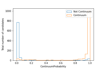
Plot the distribution of the extraInfo(ContinuumProbability) for continuum and non-continuum events, as defined by the isContinuumEvent (similarly to what was done before with R2).

Hint

Use the plotting script from the previous exercises, but with the R2 being replaced with the continuum probability.

To find out the right column name for the continuum probability, you can always check print(<yourdataframename>.columns).

Solution

# Include this only if running in a Jupyter notebook
# %matplotlib inline

import matplotlib.pyplot as plt
import uproot

var_list = ['isContinuumEvent', 'ContProb']
df = uproot.open("ContinuumSuppression_applied.root:tree").arrays(var_list, library='pd')

fig, ax = plt.subplots()

signal_df = df.query("(isContinuumEvent == 0.0)")
continuum_df = df.query("(isContinuumEvent == 1.0)")

hist_kwargs = dict(bins=30, range=(0, 1), histtype="step")
ax.hist(signal_df["ContProb"], label="Not Continuum", **hist_kwargs)
ax.hist(continuum_df["ContProb"], label="Continuum", **hist_kwargs)
ax.set_xlabel("ContinuumProbability")
ax.set_ylabel("Total number of candidates")
ax.legend()
fig.savefig("ContinuumProbability.pdf")

The resulting plot should look similar to this one:

../../_images/ContinuumProbability_uubar.png

The MVA package also has a built-in tool named basf2_mva_evaluate.py that produces several useful graphs that characterise the performance of your MVA. You can find its description at the MVA package page.

Exercise

Use the MVA evaluation function to create plots characterizing your MVA training.

Solution

Run

basf2_mva_evaluate.py -id MVAFastBDT.root \
    -train ContinuumSuppression.root \
    -data ContinuumSuppression_applied.root \
    -o evaluate.zip

This creates evaluate.zip that can be unzipped with with unzip evaluate.zip. Inside you will find the plots in pdf format and a latex.tex file that can be used to compile a single pdf that includes all the plots (see next exercise)

Warning

For the evaluation to be possible, both test and training datasets have to include all the variables that were used in the BDT training.

Exercise (optional)

If you have a running Tex distribution on your local machine, you can also generate a PDF report that includes all the plots. Note that you might have to install some additional LaTeX packages first. To generate the PDF, compile the latex.tex file from the evaluate.zip archive with a pdflatex.

There is also an option to create a pdf file straight ahead if you happen to have a basf2 installation AND all the necessary LaTeX packages on the same machine. For that you can add a -c option and run:

basf2_mva_evaluate.py -id MVAFastBDT.root \
    -train ContinuumSuppression.root \
    -data ContinuumSuppression_applied.root \
    -c -o evaluate.pdf

basf2 development documentation

Continuum Suppression (CS)

Contents

3.4.10. Continuum Suppression (CS)#

Introduction#

First Continuum Suppression steps in basf2#

Continuum suppression using Boosted Decision Trees#