3.2.2. Data Taking

Overview

Teaching: 45 min

Prerequisites:

• Fundamentals Introduction

Objectives:

• Understand the different detector systems in Belle II.

• Learn the definition of triggers and their effects.

• Know the difference between proc and prompt data processing

One of the most important steps is of course to record the data we want to analyse. In this chapter we will go through the important concepts of the Belle II detector and how we record data. Understanding these concepts is fundamental for any analysis.

The Experiment

If you are reading this manual, you are probably already at least partially familiar with the general layout of the SuperKEKB accelerator and the Belle II experiment. However, before moving on, let’s very quickly review their structure.

The SuperKEKB accelerator circulates electrons and positrons through its roughly 3 km circumference tunnel in opposite directions. These beams are asymmetric in momentum, with the electrons kept at around 7 GeV/c and the positrons at around 4 GeV/c. At a single point on the accelerator ring, the two beams are steered into (almost) head-on collision, resulting in a center-of-mass energy of typically around 10.58 GeV, corresponding to the \(\Upsilon(4S)\) resonance. The point of collision is named the “interaction region”. The center-of-mass energy can be changed to take data at other resonances of the \(\Upsilon\) family, from around 9.4 to 11 GeV, for the non-B physics part of the physics program.

Question

At the LHC, every bunch collision generates dozens of individual particle interactions that overlay each other in the detectors (pile-up), considerably complicating the data analysis. This doesn’t seem to be a problem at SuperKEKB and Belle II. Why?

Hint

Start with the planned final instantaneous luminosity of SuperKEKB. How many bunch crossings will happen per second? Then think about the typical cross sections in \(e^+e^-\) collisions as discussed previously.

Another hint

The goal instantaneous luminosity of SuperKEKB is \(6\times 10^{35}\, \textrm {cm}^{-2} \textrm{s}^{-1}\). It takes a beam particle bunch roughly 10 μs to complete a full revolution around the accelerator ring. Up to 2376 bunches will circulate in each ring.

Solution

At a final design luminosity of \(6\times 10^{35}\, \textrm{cm}^{-2}\textrm{s}^ {-1}\) at 2376 bunches per ring, each taking about 10 μs to complete a revolution, the delivered luminosity per bunch crossing is about \(6\times 10^{35}\, \textrm {cm}^{-2} \textrm{s}^{-1} \cdot 10\times 10^{-6}\ \textrm{s} / 2376 = 2.6\times10^{-6}\, (\textrm{nb})^{-1}\), so even the most likely Bhabha process at \(125\, \textrm{nb}\) only happens about once every \((2.6\times 10^{-6}\cdot 125)^{-1} \approx 3100\) bunch crossings.

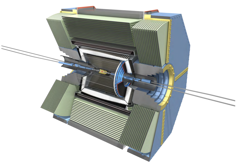
Fig. 3.3 The Belle II detector.

The detector is built around the interaction region, with the goal to detect and measure as many of the particles produced in the SuperKEKB collisions as possible. Belle II consists of several sub-systems, each one dedicated to a specific task: reconstruct the trajectory of charged track, reconstruct the energy of photons, identify the particle type or to identify muons and reconstruct long-living hadrons. Of course some systems can be used for multiple purposes: for example, the ECL is mainly intended as a device to reconstruct photons, but is also used to identify electrons and hadrons.

Due to the asymmetry of the SuperKEKB collisions, the detector is asymmetric along the beam axis. In the context of Belle II the “forward” direction is the direction in which the high energy electron beam points, while “backward” is the direction in which the lower energy positron beam points.

See also

There is an important document for any large HEP detector called the Technical Design Report (TDR). This document contains the proposed design of the experiment.

The Belle II TDR is arXiv:1011.0352.

Unfortunately, some of the details are now outdated (that document dates 2010). Particularly, we do not recommend you rely on this for performance studies.

Nonetheless you should know what it is, because people might mention it. You may need to reference it in your thesis.

Fig. 3.4 Closeup of the Belle II detector indicating all the different sub detectors.

Beam Pipe

The beam pipe itself is not an active part of the detector, but plays the crucial role of separating the detector from the interaction region, which is located in the low-pressure vacuum of the SuperKEKB rings. It is a cylindrical pipe designed to be as thin as possible in order to minimize the particle’s energy loss in it, but it is also crucial to absorb most of the soft synchrotron X-rays emitted by the beams before they can hit the detector. Otherwise they would represent a major source of noise for the innermost detector, the PXD.

PXD

The first active system met by the particles that emerge form the IP is the PiXel Detector (PXD). With this Pixel detector can measure the position of each particle going through this detector with very high precision and thus, when combining different particles, get a very precise determination where these particles intersect. This intersection is called vertex and is usually where all the particles originate from: either the place of collision or where they were created when another particle decayed.

You can think of the PXD as the inner vertex detector. The PXD is constructed from DEPFET silicon sensors segmented into individual 8 million pixels of down to 50 × 55 μm² size. It consists of two layers at 14 mm and 22 mm radius from the interaction point.

SVD

The Silicon Vertex Detector (SVD) is the outer part of the vertex detector. It comprises of double sided silicon microstrip sensors with strips widths down to 50 μm.

A double sided strip detector is similar to a pixel detector in terms of precision but we don’t have one 2D measurement of the position. Instead we have strips along the sensor on each side and measure two 1D positions: the horizontal and the vertical position on the sensor.

The four layers of the SVD system extend the outer radius of the vertex detector up to 140 mm.

VXD

You will occasionally hear people refer to the pair of detectors: PXD+SVD as the VerteX Detector (VXD). If you look at Fig. 3.5 you can see that this does make sense as both systems are closely integrated with almost no space between them. Technically they are also installed together as one unit.

Fig. 3.5 Picture of the VXD: In the middle you can see the PXD which is built around the Beam Pipe. Outside you can see the four layers of one half of the SVD.

Optional Question (hard)

This is not a question we expect you to be able to answer but it might be good to think about it for a few minutes. So here goes:

Why do we have both, a pixel and a strip detector?

Hint

Think about the differences that come from one 2D measurement vs. two 1D measurements

Answer

A strip detector measures the position of a particle by measuring vertical and horizontal position in the sensor. This means we get two measurements we can correlate to the position of the particle.

The benefit is that we have much less readout channels: instead of \(X * Y\) pixels we have \(X + Y\) strips. This means readout can be much faster and the data size will be much much smaller.

But if we have multiple particles hitting the same sensor then this can become problematic: we have to combine the horizontal and vertical measurements and for \(N\) particles passing the sensor this gives us \(N^2\) possible combinations.

So very close to the collision, where we expect the highest density of particles, it is usually much better to use a pixel detector even though the data size will be much larger.

And that’s why we have a smaller pixel detector very close to the interaction region and then a larger strip detector a bit further away.

CDC

The main tracking system for Belle II is the Central Drift Chamber (CDC). It is comprised of so-called sense wires suspended in He-C₂H₆ gas. Charged particles passing through the gas cause ionisation charges, which then drift (hence the name) to nearby sense wires, where gas amplification causes signal propagation. You will hear people refer to these ionisation signals as “hits” in the CDC.

A charged particle passing through the CDC results in a succession of hits following the trajectory of the particle. From the timing of each wire signal it is possible to infer the drift time and thus the distance at which the primary ionization was caused. You can approximate the resulting isochrone with a “drift circle” for each wire, to which the particle trajectory must have been tangent (see Fig. 3.15) . This allows for a much better point resolution than the wire spacing alone might let you assume.

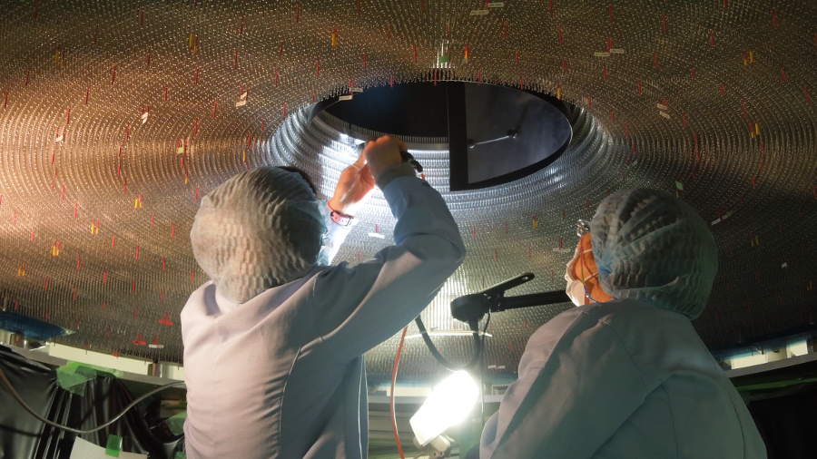
Fig. 3.6 Testing of the inner CDC wires before installation.

TOP

The Time Of Propagation (TOP) detector provides particle identification information in the barrel region of Belle II . The subdetector comprises of quartz bars and works by utilizing the Cherenkov effect. Particles passing through will cause Cherenkov photons to be emitted at an angle that directly depends on the particle velocity. Combining this velocity information with the particle momentum measured in the preceding tracking detectors yields a mass measurement, which identifies the particle species.

Emitted Cherenkov photons are captured inside the quartz bars by total internal reflection (see Fig. 3.7). TOP reconstructs the Cherenkov emission angle by measuring the effective propagation time of individual Cherenkov photons from their emissions point to the TOP sensor plane. At a given momentum, heavier particles will have lower velocities, thus a lower Cherenkov opening angle and thus, on average, a longer photon propagation path, causing a longer time of propagation of individual photons. You might also hear people refer to the TOP as the iTOP (imaging TOP).

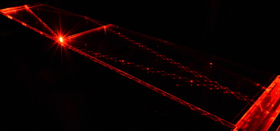
Fig. 3.7 Internal reflection of a laser inside one of the 16 bars of the TOP detector.

ARICH

The Aerogel Ring-Imaging Cherenkov detector is another dedicated particle identification subdetector using aerogel as its radiator medium. It covers the forward region of the detector.

Just as with the quartz in TOP, Cherenkov photons are emitted when a charged particle of sufficient velocity passes through the aerogel. Contrary to the TOP quartz, the aerogel does not capture the emitted Cherenkov photons, so they are forming a cone of Cherenkov light around a particle track which is imaged as a ring of characteristic radius, providing an orthogonal source of particle mass information.

Fig. 3.8 Picture of the ARICH before installation.

Question

Why is it OK to only have an ARICH in forward region and why do we not need any particle identification in the backwards direction of the detector?

Hint

Think of the beam energies at Belle II

Another hint

The nominal beam energies are 7 GeV on 4 GeV. That means the center of mass is boosted in forward direction.

Solution

The center of mass is boosted due to the asymmetric beam energies. As such, any particles generated in the collision are boosted in forward direction and the fraction of particles actually hitting the backwards direction of the detector is low.

With higher boost we would not need a backwards detector at all. And if we could go even higher with the boost we might not even need a barrel region.

So now if you look at the LHCb detector you might understand why its only a forward spectrometer: their boost is so high that they simply don’t need a barrel or backwards region at all and thus saved the money.

However they do loose hermiticity so they sacrifice the possibility to do some analysis.

ECL

The Electromagnetic Calorimeter (ECL) is chiefly tasked with measuring the electromagnetic energy of photons and electrons produced in the collision. In combination with tracking information, the calorimeter can distinguish, for example, electrons from muons.

A track from an electron will stop in the calorimeter, a muon will continue through as a minimum-ionising particle. It therefore provides further orthogonal information to the particle-identification system.

The ECL consists of over 8000 Caesium Iodide crystals which create scintillation light when a particle flies into them. The amount of light is proportional to the energy deposited in the crystal so by measuring it we can measure the energy of the the particle. Of course this assumes the particle is fully stopped and deposits all of its energy in the ECL. This is not true for most particles so we need to calibrate the light response to energy measurements.

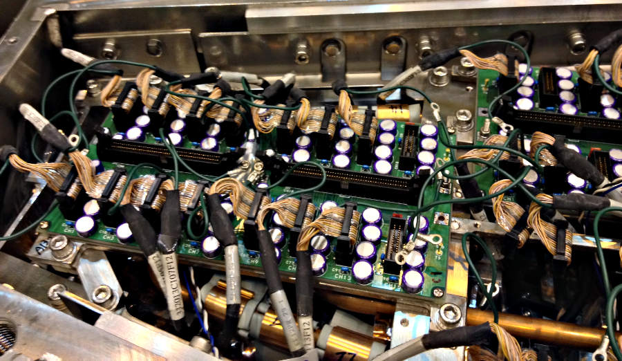
Fig. 3.9 Small part of the ECL electronics in the endcap. Boards do the mapping from the preamps (which you can’t see) to the cables that go to the ShaperDSPs. You can also see the cooling lines under the boards.

KLM

Finally, there is the KLong and Muon (KLM) system. The KLM provides muon identification information to tracks that pass through all other subdetectors and also reconstructs \(K_L^0\) s from the collision.

See also

There are two more useful reference documents that you should be aware of. Now seems like a good time to mention them.

1. Bevan, A. et al. The Physics of the B Factories. Eur.Phys.J. C 74 3026(2014). https://doi.org/10.1140/epjc/s10052-014-3026-9

2. Kou, E. et al. The Belle II physics book, PTEP 2019 12 123C01, https://doi.org/10.1093/ptep/ptz106.

The former is a book describing the previous generation B-factories (the detectors and their achievements). The latter describes the Belle II detector and the physics goals. It is sometimes referred to (rather opaquely) as the B2TiP report. If you are a newcomer you should probably refer to it as it’s (significantly more sane) official name.

Key points

• You have heard of all the sub detectors and what their primary measurement is

• You know where to find the Belle II TDR, “The Physics of the B factories”, and “The Belle II physics book”.

On Resonance, Continuum, Cosmics

We saw that to collect \(B\) mesons one must collide electrons and positrons at the center-of-mass energy of \(\sqrt{s} = 10.580\) GeV, corresponding to the \(\Upsilon(4S)\) resonance mass. However this is not the only energy at which the SuperKEKB accelerator can work, and it’s not the only kind of dataset that Belle II can collect.

On-resonance

The standard collisions at \(\sqrt{s} = 10.580\) GeV.

Off-resonance

\(e^+e^- \to \Upsilon(4S) \to B\bar{B}\) is not the only process that takes place at \(\sqrt{s} = 10.580\) GeV. The production of light and charm quark pairs in the reaction \(e^+e^- \to u\bar{u}, d\bar{d}, s\bar{s}, c\bar{c}\) has a total cross section of about \(3.7\) nb is more that three times larger than the production of \(B\) mesons. As the quarks hadronize leaving final states that are similar to the \(B\bar{B}\). This background can be studied using the Monte Carlo simulation, but it’s more effective to study it directly on data. Occasionally, 1–2 times per year, a special dataset is collected approximately 60 MeV below the \(\Upsilon(4S)\). Here no \(B\) mesons can be produced, leaving one with a pure sample of continuum events, called off-resonance (or continuum) sample.

Fig. 3.10 Cross section around the Υ resonances showing the difference between on- and off-resonance.

Cosmic

At the beginning and end of each run period Belle II acquires cosmic muons. These events are used mainly for performance studies and for calibration, as they provide an unique sample for aligning the detectors with each other. Usually part of this dataset is collected with the solenoid switched off, so that muons cross the detectors on straight trajectories. If the SuperKEKB accelerator has a major downtime of few days, a cosmic dataset is usually collected to keep the Belle II system running.

Beam

Beam runs are special, usually short data takings used to study the beam-induced background on the inner sub-detectors. They are taken with the beams circulating without colliding, to remove all the processes related to \(e^+e^-\) hard scattering.

Scan

A scan consists of rather short data taking periods (hours or few days long) performed at slightly different energies (usually 10–50 MeV apart). The goals of a scan is to measure the line shape of the \(e^+e^-\) cross section to either check that data are collected on the resonance peak (short scans), or to perform real physics measurements such as the search for exotic vector resonances (long scans above the \(\Upsilon(4S)\) energy).

Non-4S

SuperKEKB can operate across the whole spectrum of bottomonia, from the \(\Upsilon(1S)\) at \(9.460\) GeV to slightly above the \(\Upsilon(6S)\) at around \(11.00\) GeV. These datasets can be used for all the non-B parts of the Belle II physics program, but are particularly interesting for the spectroscopy, hadronic physics and dark sector studies.

Triggers and filters

SuperKEKB bunches can cross the interaction region up to every 4 ns. However, in the vast majority of cases either no collision (more precisely: no hard interaction) takes place at all, or the collision results are not interesting (for example \(e^+e^-\to e^+e^-\) events are the most common, but of secondary interest to our physics program).

Recording and keeping all detector information for each collision would be wasteful. Not only are most events not interesting, but the bandwidth requirements to the offline disks would be impossible to provide. Like most HEP experiments we therefore trigger and filter events. This is all achieved with the Belle II online system (you might hear people refer to it as “online”). The online system consists of the Data Acquisition (DAQ), Level 1 Trigger (TRG, also called L1) and the High Level Trigger (HLT). These two trigger systems are designed to reduce the amount of data as much as possible before they reach the first storage hard disk.

Generally, when Belle II is running and operational, each subdetector will transmit its readout data upon receipt of an external trigger signal. The data gathered from all subdetectors in response to a given external trigger is what we call “one event”. Generating this trigger signal for each “interesting” collision is the task of the TRG system. The TRG system receives what effectively amounts to a low resolution “live stream” of the readout data of CDC, ECL and KLM (for completeness: TOP also sends stream data to TRG but it is not used for triggering directly). The streamed data is interpreted in near realtime using specialized fast electronics (Field Programmable Gate Arrays, FPGAs) by continuously matching it to predefined trigger conditions. If TRG determines an interesting collision event has just taken place, it generates a trigger signal which is distributed to all subdetectors. The TRG system is designed to issue up to 30 kHz of such triggers at the full SuperKEKB design luminosity.

Note

The TRG system will issue a trigger decision with a fixed delay of about 4 µs. In practice, all subdetector frontend electronics thus have to keep a buffer of their readout data of the past several microseconds, so they can transmit the measurement they took in the time slice around 4 µs ago.

The DAQ system makes sure that all trigger signals are synchronously delivered to all subdetectors. It also provides the high-speed data links that are used to read out the subdetector data for each event and forwards it to the HLT system.

Fig. 3.11 Simplified diagram of the Belle II data flow.

The HLT system is a computing cluster of about 10000 CPU cores located right next to the detector. It receives the full raw subdetector data for each triggered event and performs an immediate full reconstruction using the exact same basf2 software as is used in offline data analysis. Based on the result of this reconstruction, events are classified and either stored to a local offline storage hard disk drive or discarded. This high level event selection is expected to reduce the amount of data written to the offline storage by at least 60%.

Note

The HLT can operate in two modes: filtering and monitoring. In the former the events that do not satisfy any of the HLT selections (called “lines”) are discarded and lost forever. In the latter, all the events are kept regardless of the HLT decision (which is however stored, so analyses of the HLT filtering efficiency can be conducted). On top of this, the HLT also performs a first, rough skimming producing the so-called HLT skims. All the events that are satisfying the HLT conditions (regardless of the HLT operation mode), are then assigned according to a quick analysis into few possible categories: bhabha, hadronic, tau, mumu and so on attaching a flag to them, which can then be read out from the raw data without reconstructing the full event. This categorization is mainly done to quickly select the events that are needed for calibration and send them to the calibration center, however the hadronic HLT skim (called hlt_hadron) has become increasingly popular to perform analysis in the early stage of the experiment, and is being considered as a starting point for many analysis skims (more on them later), so you will likely hear of it.

Fig. 3.12 The HLT is one of the critical parts of our data taking chain. Every part of it needs to be carefully installed, maintained, and operated.

Both the TRG system and the HLT classify events based on the data available to them. While the decision whether to issue a trigger for a given collision (or on HLT whether to keep the event or discard it) is of course binary, certain event classes might be intentionally triggered at less than 100% of their occurrence. For example, while Bhabha scattering events (\(e^+e^- \to e^+e^-\), often just called “Bhabhas”) are generally not very interesting for the physics program of Belle II, keeping some of them for calibration purposes might be very useful. Since Bhabhas are easily identified even with the limited information available to the TRG system, the TRG system will not issue a trigger for every single identified Bhabha event, but only for a configurable fraction. This technique of intentionally issuing triggers only for fractions of a given event class is named prescaling. When working on your own analysis, it is very important to keep in mind potential prescaling of the triggers that yield the events you use in your analysis. Since the prescaling settings can (and will) change over the lifetime of the experiment, updated numbers for each run can be found here.. See also this question. for more details.

Since the TRG and HLT systems are ultimately deciding which data is being kept for offline analysis, understanding and validating their performance vs. their intended functionality is of highest importance for the success of the experiment.

Key points

• The TRG system aims to recognize interesting events from the near continuous stream of collisions.

• The HLT system uses the full readout data for each event to further decide which events to keep for offline analysis and which ones to discard.

• Prescaling might be used to only record every n-th event (on average) that satisfies given trigger conditions.

Processing Data Samples

Data from physics runs undergo two main stages of processing: prompt processing and reprocessing. The difference between them relates to the level of calibrations that are applied during the processing. The relationship between each stage of processing (described below) is represented schematically in Fig. 3.13.

Prompt processing occurs just after the data taking. Data is collected for a given amount of time, typically two weeks (colloquially called a “bucket”), then it is calibrated and processed, and then the process is iterated. Prompt data is always obtained using the latest major software release, and its calibration is complete, with quality that is hardly different from the reprocessed data. For this reason, most of the calibration performed in prompt is kept also for reprocessing. Prompt data is available for analysis after prompt processing, with a timescale of about 2 months.

During a reprocessing, all data collected up to a given time is recalibrated and reprocessed. A reprocessing campaign, labelled with the prefix “proc” (e.g. proc13), is done every year or every two years (from 2023). The recalibration starts from the prompt calibration, and it is refined if improved or new calibration algorithms were developed. A full reprocessing of data is performed using a major software release, so that the complete dataset is available with a coherent processing.

Both prompt and reprocessed datasets can be accessed on the grid using the corresponding collections reported on the Data Production web page.

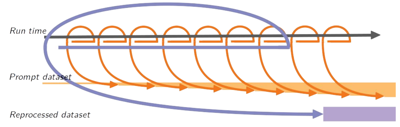
Fig. 3.13 A diagram showing the relationship between data collected at run time, prompt datasets, showing the incremental processing and reprocessed data (e.g. procXX).

Stuck? We can help!

If you get stuck or have any questions to the online book material, the #starterkit-workshop channel in our chat is full of nice people who will provide fast help.

Refer to Collaborative Tools. for other places to get help if you have specific or detailed questions about your own analysis.

Improving things!

If you know how to do it, we recommend you to report bugs and other requests with GitLab. Make sure to use the documentation-training label of the basf2 project.

If you just want to give very quick feedback, use the last box “Quick feedback”.

Please make sure to be as precise as possible to make it easier for us to fix things! So for example:

• typos (where?)

• missing bits of information (what?)

• bugs (what did you do? what goes wrong?)

• too hard exercises (which one?)

• etc.

If you are familiar with git and want to create your first merge request for the software, take a look at How to contribute. We’d be happy to have you on the team!

Quick feedback!

Author(s) of this lesson

Umberto Tamponi, Martin Ritter, Oskar Hartbrich, Michael Eliachevitch, Sam Cunliffe, Priyanka Cheema, Stefano Lacaprara