
3.3.3. Python#
High Energy Physics (HEP) analyses are too complex to be done with pen, paper and calculator. They usually are not even suited for spreadsheet programs like Excel. There are multiple reasons for this. For one the data size is usually larger than paper or spreadsheets can handle. But also the steps we take are quite complex. You are of course welcome to try but we really don’t recommend it.
So what we need is something more powerful. For many years the HEP community believed that only very fast and complex programming languages are powerful enough to handle our data. So most students needed to start with C++ or even Fortran.
And while there’s nothing wrong with those languages once you mastered them, the learning curve is very long and steep. Issues with the language have been known to take a major fraction of students time with frustrating issues like:
Why does it not compile?
It crashes with an error called “segmentation violation”, what’s that?
Somehow it used up all my memory and I didn’t even load the data file yet.
And while it’s true that once the program was finally done running the analysis be very fast it is not necessarily efficient. Spending half a year for on a program for it to finish in an hour instead of one month development and have it finish in a day is maybe not the best use of students time.
So in recent years HEP has started moving to Python for analysis use: It is very easy to learn and has very nice scientific libraries to do all kinds of things. Some people still say python is way too slow and if you misuse it that is certainly true. But if used correctly python is usually much easier to write and can achieve comparable if not better speeds when compared to naive C++ implementations. Yes, if you are a master of C++ nothing can beat your execution speed but the language is very hard to master. In contrast Python offers sophisticated and optimized libraries for basically all relevant use cases. Usually these include optimizations that would take years to implement in C++, like GPU support.
Think about it: almost all of the billion dollar industry that is machine learning is done in Python and they would not do that if it would not be efficient.
Consequently in Belle II we make heavy use of Python which means you will need to be familiar with it. By now you probably know what’s coming next.
Luckily there is a very large amount of good python tutorials out there. We’ll stick with Software Carpentry and their Programming with Python introduction. We would like you to go there and go through the introduction and then come back here when you are done.
What are the key concepts of python?#
See also
While we’d encourage you to work through this section by yourself, we’ve also prepared a video to help. Please stop it at every exercise to think and try to do all steps by yourself as well.
Welcome back! Now we’re going to test you on your new-found knowledge in Python.
As you should be aware by now, the key concepts of python include:
importing libraries that you wish to use
importing and/or storing data in different ways i.e. arrays, lists
writing and using (sometimes pre-defined) functions
writing conditions: if statements, for loops etc.
understanding and using errors to debug
You should be aware that there are multiple ways of running python. Either interactively from your terminal:
python3
As a script from your terminal:
python3 my_script.py # where this file has python commands inside
Or within a python compiler and interpreter such as Visual Studio or XCode.
The official recommended version of python is python3. Python2 is no longer supported. To check which python version you have installed you can check in your terminal using
python3 --version
OR you could perform this in a live python session, either in your terminal or in a jupyter notebook using:
from platform import python_version
print(python_version())
Let’s create a python file from terminal and run it
Exercise
Log in to KEKCC. Create a folder starterkit in your home folder and
create a python file my_file.py. Import the basic math library math
and print out the value of π.
Hint
To create a file you’ll need to use your bash skills. The internet is your friend.
Hint
The specific bash commands you’ll need are mkdir, cd and touch.
Hint
Add the import command inside your python file using your favorite
editor. Previous tutorials introduced the nano editor to you.
Solution
# Make sure we're in our home directory
cd ~
# Create a folder and change there
mkdir starterkit
cd starterkit
# Create your .py file
touch my_file.py
# Open your file to edit it in your editor of choice, e.g.
nano my_file.py
Now add the python lines to your file.
Congratulations! You’ve now created your first python file. Now, run it!
Exercise
Run your new python file in your terminal.
Solution
python3 my_file.py
Great! Well done! 😁 You can now create python scripts in your terminal!
Practising Python: Jupyter notebooks#
See also
While we’d encourage you to work through this section by yourself, we’ve also prepared a video to help. Please stop it at every exercise to think and try to do all steps by yourself as well.
We will work in a jupyter notebook to allow you to practice using your python skills further.
Jupyter Notebooks are interactive notebooks that allow one to visualise code, data and outputs in a very simple way. When you run a notebook you have an operating system called a kernel that runs the code.
Exercise
Navigate to your starterkit folder on KEKCC that you created in the previous
exercise. Start your Jupyter notebook server. Open the jupyter page in your browser.
Solution
cd ~/starterkit  # just to make sure we're there
jupyter-notebook --port <your forwarded port> --no-browser
Connecting and starting a jupyter notebook is described in more detail here (SSH - Secure Shell).
Running on other servers (optional)
In principle most of the content of this page will work from anywhere if you have installed the right packages.
If you have the Belle II software explained and set up, there are no issues at all. Please start your jupyter notebook after running
b2setupas shown in the SSH tutorialIf you are using the DESY NAF Jupyter Hub, make sure that you select the latest Belle II software release as kernel (i.e.
release-xx-xx-xx), rather thanpython(the letter won’t have ROOT properly set up).If you cannot set up the Belle II software, you might need to install some packages locally
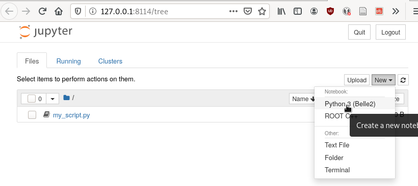
Note that your script my_script.py from before is also shown.
Exercise
Click on my_script.py and add another line of python code and save.
Go back to the home screen and click on “New” and then “Text File”.
Call your file my_second_script.py and add a couple of lines of
python.
Exercise
Now open a second terminal window and connect to kekcc. Verify that you did indeed create the second file and change the contents of the first.
Solution
cd ~/starterkit
ls
cat my_script.py
cat my_second_script.py
Hint
Throughout all of the following lessons you always need to have one terminal window for your jupyter notebook to run in and one more to enter commands in bash, just as we practiced right now.
Okay, so we can also create and edit files through our browser. Nice!
But the true power of jupyter are its notebooks. Click on “New” and “Python 3 (Belle 2)” as shown in the screenshot
A new window with your notebook will open.
The main difference between using a jupyter
notebook (.ipynb) and a python file (.py) is that jupyter notebooks
are interactive and allow you to see what your code does each step of
the way. If you were to type all of code into a python
file and run it, you would achieve the same output (provided you save
something as output).
Each block in a jupyter
notebook is a “cell”. These cells can be run using the kernel by clicking the
run button or by pressing Shift + Enter. When you run a cell, the kernel will
process and store any variables or dataframes you define. If your kernel
crashes, you will have to restart it.
Exercise
Click on “Help” and then on “User Interface Tour” to get a first overview
over jupyter.
Examine the Cell and Kernel drop down menus to see what options
you have available.
Exercise
Write a couple of lines of python in a cell of the notebook and execute them.
It is also useful to be able to access help or extra information about the
tools you will be using. In particular you will often want to check
information about a python object you are using. The definition of a python
object includes commands, packages, modules, classes, types…
basically anything that has a description called a docstring).
There are multiple ways to access this information, including
what is already discussed in The basics.
For jupyter notebooks, a great interactive way to access the information
(docstring) is by putting your cursor on the object in question and pressing
Shift + Tab.
In addition to the Shift + Tab option, you can also run a cell with your
object in question, with a question mark! For example, if our object in
question is the print function we can type:
print?
For any python interpreter, one can also use:
Pandas Tutorial and Python Data Analysis#
This section aims to answer the question “How can I process tabular data?”
We will use the uproot package to read TTrees from ROOT files.
Now, the previous sentence may have not been familiar to you at all. If so, read on. If not, feel free to skip the next paragraph.
ROOT: a nano introduction#
ROOT files, as you’ll come to be familiar with, are the main way we store our
data at Belle II. Within these files are TTree objects known as trees, which are
analogous to a sub-folder. For example, you may store a tree full of \(B\)
meson candidates. Within a tree you can have TBranch’es known as
branches. Each branch could be one of the oodles of variables available for
the particle you’ve stored in your tree — for example, the \(B\) meson’s
invariant mass, it’s daughter’s momentum, it’s great-great-granddaughter’s
cluster energy etc. etc. etc.
More information: CERN’s ROOT
If you get stuck with ROOT, you can also ask in CERN’s ROOT Forum
Importing ROOT files#
In this section we will learn how to import a ROOT file as a Pandas DataFrame
using the uproot library. No ROOT installation is necessary for this to work!
Pandas provides high-performance, easy-to-use data structures and data analysis tools for Python, see here.
Exercise
Start a new notebook and import uproot.
Solution
import uproot
You can load in an example file using the open function from the uproot package.
file_path = "https://rebrand.ly/00vvyzg"
file = uproot.open(file_path)
This code imports the pandas_tutorial_ntuple.root root file as a file object file.
For speed it is beneficial to download the file first and pass the path to your local copy to uproot.open.
You are welcome to import your own root files, but be aware that the variables and outputs will appear differently to this tutorial.
The keys method lists the tree(s) in that file. file behaves much like a dictionary in that you can access the trees like you would access values in a dictionary.
print(file.keys())
tree = file["b0phiKs"]
Shortcut to reading trees
If you already know the contents of the file, i.e. the name of the tree you want to read (in our case "b0phiKs"), you can get it in one go by passing the name of the tree after a colon to the open method.
tree = uproot.open(file_path + ":b0phiKs")
Automatic closing of open file
In a python script it is good practice to open files in a with-block. Uproot supports this too.
with uproot.open(file_path + ":b0phiKs") as tree:
  ...
This construct guarantees that the file will be closed properly, even if the program crashes due to exceptions.
Uproot is only responsible for reading and writing ROOT files, it does not contain any functionality to perform computations on the data. For this, we need to read the data into a pandas DataFrame. In uproot, there are two different ways to do this.
The first option is to load all events at once with the arrays method:
df = tree.arrays(library="pd")
The library="pd" parameter tells uproot that we want to get back a pandas DataFrame. If you rather not work with pandas, uproot also supports numpy ("np") and
awkward array ("ak").
Note that this loads the entire tree into memory at once, so keep that in mind when trying to load very large files. If you run into memory problems,
the second option to load data from a tree is with the iterate method, discussed in section Dealing with large / many files (optional).
TL;DR
load a tree
tree = uproot.open(filename + ":" + treename)
df = tree.arrays(library="pd")
or
with tree as uproot.open(filename + ":" + treename):
  df = tree.arrays(library="pd")
Note about speed
If you have a workflow that uses modularAnalysis.variablesToNtuple() to create NTuples and you observe very slow
loading times when reading those NTuples with uproot, this is probably due to small basket sizes in the output NTuples.
To change this, set the basketsize parameter of the modularAnalysis.variablesToNtuple() method to a large number
(eg. 20000000). The produced NTuples should then be faster to read in uproot.
As a general rule of thumb about the size of this number: make sure that the basketsize times the number of branches you want
to read at once is smaller than the available memory of your machine.
Investigating your DataFrame#
In jupyter notebooks, the last value of a cell is shown as output. So if we create a cell with
df
as the last line, we will see a visual representation of the dataframe. In your case each row of the dataframe corresponds to one candidate of a collision event.
You can also show a preview of the dataframe by only showing the first few rows using head.
Similarly tail shows the last few rows. Optionally: You can
specify the number of rows shown in parentheses.
df.head(5)
Each DataFrame has an index (you can think of this as row numbers, in our case the number of the candidates) and a set of columns:
len(df.columns)
You can access the full data stored in the DataFrame with the to_numpy method,
which is a large 2D numpy matrix
df.to_numpy
However to_numpy may not be the most visually pleasing (or easy) way to inspect the contents of your dataframe.
A useful feature to quickly summarize your data is to use the describe method:
df.describe()
Exercise
What are the output rows of df.describe?
Hint
No hint here!
Solution
df.describe has the great ability to summarize each of your columns/variables. When using it, a table is printed with rows of ‘count’, ‘mean’, ‘std’, ‘min’, ‘25%’, ‘50%’, ‘75%’ and ‘max’.
count, the number of entriesmean, the average of all entriesstd, the standard deviation of the columnmin, andmax: the smallest and largest value of the column25%,50%,75%: the value where only 25%, 50% or 75% of the entries in the column have a smaller value. For example if we have 100 entries in the dataframe the 25% quantile is the 25th smallest value. The 50% quantile is also known as the median.
You can also display the values of the DataFrame sorted by a specific column:
df.sort_values(by='B0_M').head()
Finally, everyone who works with numpy and pandas will at some point try to use a fancy function and get an error message that the shapes of some objects differ.
Exercise
What is the output of df.shape and what does it mean?
Hint
Try it out in your jupyter notebook. To understand the output, df.shape? (or pd.DataFrame.shape?) is,
once again, your friend.
Solution
The output comes in the form of a tuple (a finite ordered list (or sequence) of elements). For example, one output could be (15540523, 20), which is saying you have a dataframe of 15540523 rows, and 20 columns.
Selecting columns#
Selecting a column can be performed by df['column_name'] or
df.column_name. The result will be a pandas Series, a 1D vector. The
difference between the two options is that using df.column allows for
auto-completion.
df['B0_M'].describe()
# or
df.B0_M.describe()
Multiple columns can be selected by passing an array of columns:
df[['B0_mbc', 'B0_M', 'B0_deltae', 'B0_isSignal']].describe()
We can assign this subset of our original dataframe to a new variable
subset = df[['B0_mbc', 'B0_M', 'B0_deltae', 'B0_isSignal']]
subset.columns
Selecting Rows#
Similarly to arrays in python, one can select rows via df[i:j]. And single
rows can be returned via df.iloc[i].
df[2:10]
Vectorized Operations#
This is one of the most powerful features of pandas and numpy. Operations on a Series or DataFrame are performed element-wise.
df.B0_mbc - df.B0_M
Let’s look a slightly more complicated (but totally non-physical) example:
Adding Columns#
You can easily add columns in the following way:
df['fancy_new_column'] = (df.B0_deltae * df.B0_et)**2 / np.sin(df.B0_cc2)
df['delta_M_mbc'] = df.B0_M - df.B0_mbc
df.delta_M_mbc.describe()
df['fancy_new_column']
Modifying Columns#
Sometimes we want to change the type of a column. For example if we look at all
the different values in the B0_isSignal column by using
df['B0_isSignal'].unique()
we see that there are only two values. So it might make more sense to interpret this as a boolean value:
df['B0_isSignal'] = df['B0_isSignal'].astype(bool)
df.B0_isSignal.value_counts()
Querying Rows (i.e. making cuts)#
Finally, arguably the most useful function for your analyses is the query function. Querying allows one to cut on data using variables and values using a ‘cut string’. Within your cut string you can use usual python logic to have many arguments. For example:
df.query("(B0_mbc>5.2) & (B0_deltae>-1)")
Exercise
Create two DataFrames, one for Signal and one for Background only
containing B0_mbc, B0_M, B0_isSignal and B0_deltae columns.
Hint
Split between signal and background using the B0_isSignal column.
Solution
bkgd_df = df.query("B0_isSignal==0")[["B0_mbc", "B0_M", "B0_isSignal", "B0_deltae"]]
signal_df = df.query("B0_isSignal==1")[["B0_mbc", "B0_M", "B0_isSignal", "B0_deltae"]]
Grouped Operations: a quick note#
One of the most powerful features of pandas is the groupby operation. This
is beyond the scope of the tutorial, but the user should be aware of it’s
existence ready for later analysis. groupby allows the user to group all
rows in a dateframe by selected variables.
df.groupby('B0_isSignal').describe()
A short introduction to plotting in python#
In this section we will answer “How can I plot data?” and demonstrate the matplotlib package used to plot in python.
import matplotlib.pyplot as plt
# show plots in notebook
%matplotlib inline
Hint
%matplotlib inline is not normal python code (you might get a SyntaxError), but a so called
magic function
of your interactive python environment. Here it is responsible for showing the
plots in your notebook.
If you don’t see any plots, you have probably forgot to include and execute this line!
In previous example workshops the simple decay mode \(B^0\to \phi K_S^0\),
where \(\phi \to K^+ K^-\) and \(K_S^0 \to \pi^+ \pi^-\) was
reconstructed. Now we will use these candidates to plot example
distributions. We use the uproot package to read the data
import uproot

file_path = "https://rebrand.ly/00vvyzg"
df = uproot.open(file_path + ":b0phiKs").arrays(library="pd")
df.B0_isSignal = df.B0_isSignal.astype(bool)
df.describe()
Pandas built in histogram function#
There exists, if you prefer, a built in histogram function for Pandas. The following cells show how to implement it.
df.B0_mbc.hist(range=(5.2, 5.3), bins=100)
df.B0_mbc.hist(range=(5.2, 5.3), bins=100, by=df.B0_isSignal)
df.query("B0_isSignal==1").B0_mbc.hist(range=(5.2, 5.3), bins=100)
df.query("B0_isSignal==0").B0_mbc.hist(range=(5.2, 5.3), bins=100, alpha=.5)
Exercise
Now plot B0_deltae separately for signal and background.
Using Matplotlib#
Internally the pandas library however makes use of matplotlib itself. Using matplotlib directly opens up many more possibilities. It also works well with juptyer notebooks, so this is what this tutorial will focus on. Compare the following two code snippets with their equivalent of the last section to get a feeling for the syntax.
h = plt.hist(df.B0_mbc, bins=100, range=(5.2, 5.3))
h = plt.hist(df.query("B0_isSignal==1").B0_mbc, bins=100, range=(5.2, 5.3))
h = plt.hist(df.query("B0_isSignal==0").B0_mbc, bins=100, range=(5.2, 5.3))
Making your plots pretty#
Let’s face it, physicists aren’t well known for their amazing graphical representations, but here’s our chance to shine! We can implement matplotlib functions to make our plots GREAT. You can even choose a colourblind friendly colour scheme!
It is possible to display multiple plots at once using plt.subplots. As you can see
below, rather than simply having our histograms show up using plt, we define a
figure fig and axes ax.
These are the equivalent of our canvas where we paint our code art.
# Here we set up the "canvas" to show two plots side by side
fig, ax = plt.subplots(nrows=1, ncols=2, figsize=(10, 6))
# ax is now an array with two elements, each representing one plot

h = ax[0].hist(df.query("(B0_isSignal == 1)").B0_mbc, bins=100, range=(5.2, 5.3),
              histtype='stepfilled', lw=1, label="Signal", edgecolor='black')
h = ax[1].hist(df.query("(B0_isSignal == 0)").B0_mbc, bins=100, range=(5.2, 5.3),
              histtype='step', lw=2, label="Background")

ax[0].legend(loc="best")
ax[0].set_xlabel(r"$M_{\mathrm{bc}}$", fontsize=18)
ax[0].grid() # applies a nice grid to the plot
ax[0].set_xlim(5.2, 5.3) # sets the range of the x-axis

plt.show()  # shows the figure after all changes to the style have been made
Note
Note that we were using so-called r-strings: r"this is my string".
Usually characters escaped with a backslash have special meanings. For example
\n represents a line break. If you want to type a literal \n (for example
when you type a \(\nu\) in LaTeX for your plot labels as \nu), you can either
“escape” the backslash \\nu or deactivate special characters altogether by
adding an r to the beginning of the string r"\nu".
Exercise
Run the above code to see the effects on the output and then apply your own changes to the second axis.
Hint
ax[0] refers to the first axis, so all changes in the code snippet above will
only change that axis.
Solution
This solution is a basic example, there are many fun style edits you can find online for yourself.
fig, ax = plt.subplots(1,2,figsize=(10,6))

h = ax[0].hist(df.query("(B0_isSignal == 1)").B0_mbc, bins=100, range=(5.2, 5.3),
              histtype='stepfilled', lw=1, label="Signal", edgecolor='black')
h = ax[1].hist(df.query("(B0_isSignal == 0)").B0_mbc, bins=100, range=(5.2, 5.3),
              histtype='step', lw=2, label="Background")

ax[0].legend(loc="best")
ax[1].legend(loc=3)

ax[0].set_xlabel(r"$M_{\mathrm{bc}}$", fontsize=18)
ax[1].set_xlabel(r"$M_{\mathrm{bc}}$", fontsize=20)

ax[0].grid()

ax[0].set_xlim(5.2, 5.3)
ax[1].set_xlim(5.2, 5.3)

plt.show()
The implementation of 2D histograms are often very useful and are easily done:
plt.figure(figsize=(15,10))
cut = '(B0_mbc>5.2) & (B0_phi_M<1.1)'
h = plt.hist2d(df.query(cut).B0_mbc, df.query(cut).B0_phi_M, bins=100)
plt.xlabel(r"$M_{BC}$")
plt.ylabel(r"$M(\phi)$")
plt.savefig("2dplot.pdf")
plt.show()
Note
Note here how the query cut has been defined as the string cut which is then
passed to df.query. You should always avoid copy/pasting the same code
(inflexible and prone to errors).
Exercise
However the code above is not as efficient as it could be. Do you see why? How could you solve this?
Hint
With a very large dataframe, query can take a lot of time (you need to look
at every row of the dataframe, even if only few rows pass the selection)
Hint
So the issue is that you call df.query(cut) twice. How could you avoid this?
Solution
You could simply define df_cut = df.query(cut) and then use df_cut
in line 3.
Another way to use matplotlib with dataframes
Most matplotlib functions also support a data keyword which can take a
dataframe. Afterwards you can specify columns by their string names.
In our example, line 3 could have been
h = plt.hist2d("B0_mbc", "B0_phi_M", bins=100, data=df.query(cut))
Note that this also solves the last exercise (we only call query once).
Finally, Belle II does have an official plot style, for plots that are published internally and externally. You do not need to worry about this at this stage, but keep it in mind.
Warning
The following will only work if you have the Belle II software basf2 set up.
You will learn how to do so in the following chapters.
You’re invited to still try executing the following lines, but don’t worry if
you see an error message telling you that the style has not been found.
Importing the style is as easy as “one, two, …
from matplotlib import pyplot as plt
plt.style.use("belle2")
See also
A very fun way to explore the capabilities of matplotlib is the
matplotlib gallery that
shows many example plots together with the code that was used to generate them.
Exercise
Select your favorite plot from the matplotlib gallery. Can you generate
it in your notebook? Try to modify some properties of the plotting
(different colors, labels or data).
Solution
You should be able to generate the picture simply by copy-pasting the code example given.
Dealing with large / many files (optional)#
If your files are quite large you may start to find your program or jupyter notebook kernel crashing - there are a few ways in which we can mitigate this.
“Chunk” your data
Only import the columns (variables) that you will use/need.
To import the file using chunking, instead of loading the tree with the arrays method, we can iterate over chunks of the tree with the iterate method.
for df in tree.iterate(Y4S_columns, step_size=100_000, library="pd"):
  ...
Here a few columns have been defined which are included in the following list:
Y4S_columns = ['B0_mbc', 'B0_M', 'B0_deltae', 'B0_isSignal']
Exercise
Load your dataframe as chunks of 100000 events.
Solution
file = "https://rebrand.ly/00vvyzg"
tree = uproot.open(file + ":b0phiKs")
for df_chunk in tree.iterate(Y4S_columns, step_size=100_000, library="pd"):
  ...
Now the data is loaded as chunks, we “loop” over or run through all the chunks and perform selection and further processing on those chunks instead of on the whole dataset at once.
You can read more about the many features of the iterate method in the documentation.
If you want to process many files, uproot offers the function uproot.iterate so you don’t have to loop manually over all files. It has a similar interface to the tree methods arrays and iterate,
except it also accepts a list of files or a wildcard expression:
for df_chunk in uproot.iterate("data/signal*.root:tree", columns, step_size=100_000, library="pd"):
  ...
Your journey continues#
If you haven’t programmed in python before this lesson, then you’re probably quite exhausted at this point and deserve a break!
However, your python journey has just begun and there’s a lot to learn.
Hint
Even if you can somehow get your analysis “to work” with your current understanding of python, we can’t encourage you enough to keep on educating yourself about python and its best coding practices.
Chances are you will write a LOT of code and work on your analysis for a long time. Bad design decisions and sloppy coding practices will slowly build up and might cost you a lot of time and nerves in the end (and will cause pain to anyone who will have to work with your code afterwards).
I promise I will read more about this.
Exercise
A small easter egg that has been included in python: Simply run
import this
Can you make sense of the output?
Solution
This “Zen of Python” collects 19 guiding principles for writing good python code. There’s a wikipedia page about it and many more resources that you can google that go into more detail.
See also
We have started to compile a reading list for python on XWiki. Please help us extend it!
Stuck? We can help!
If you get stuck or have any questions to the online book material, the #starterkit-workshop channel in our chat is full of nice people who will provide fast help.
Refer to Collaborative Tools. for other places to get help if you have specific or detailed questions about your own analysis.
Improving things!
If you know how to do it, we recommend you to report bugs and other requests
with GitLab.
Make sure to use the documentation-training label of the basf2 project.
If you just want to give us feedback, please open a GitLab issue and add the label online_book to it.
Please make sure to be as precise as possible to make it easier for us to fix things! So for example:
typos (where?)
missing bits of information (what?)
bugs (what did you do? what goes wrong?)
too hard exercises (which one?)
etc.
If you are familiar with git and want to create your first merge request for the software, take a look at How to contribute. We’d be happy to have you on the team!
Quick feedback!
Do you want to leave us some feedback? Open a GitLab issue and add the label online_book to it.
Authors of this lesson
Martin Ritter (Intro), Hannah Wakeling (Exercises), Kilian Lieret