7.8.5. Full event interpretation#

Algorithm overview#

Physics#

Measurements of decays including neutrinos, in particular rare decays, suffer from missing kinematic information. The FEI recovers this information partially and infers strong constraints on the signal candidates by automatically reconstructing the rest of the event in thousands of exclusive decay channels. The Full Event Interpretation (FEI) is an essential component in a wide range of important analyses, including: the measurement of the CKM element $|V_{ub}|$ through the semileptonic decay $b \rightarrow u \nu$; the search for a charged-Higgs effect in $B \rightarrow D \tau \nu$; and the precise measurement of the branching fraction of $B \rightarrow \tau \nu$, which is sensitive to new physics effects.

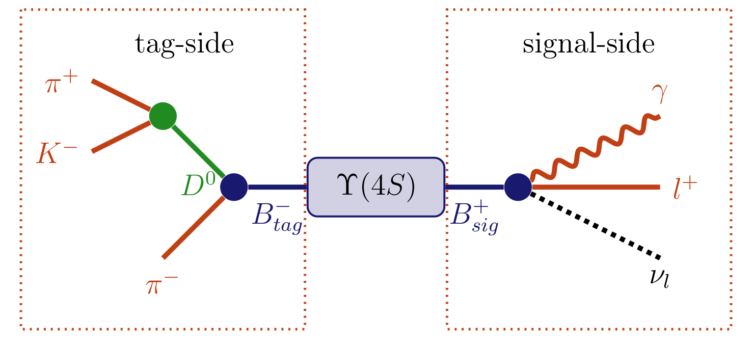
../../_images/example_decay.png — Fig. 7.5 $\Upsilon(4S)\rightarrow (B^{+} \rightarrow l^{+} \nu_{l} \gamma) (B^{-} \rightarrow (D^{0} \rightarrow K^{-} \pi^{+}) \pi^{-})$ decay topology. Here the decay $B^{-} \rightarrow (D^{0} \rightarrow K^{-} \pi^{+}) \pi^{-}$ can be reconstructed as the tag-side allowing additional information about the signal-side $B^{+} \rightarrow l^{+} \nu_{l} \gamma$ to be deduced.#

As an analysis technique unique to B factories, the Full Event Interpretation will play an important role in the measurement of rare decays. This technique reconstructs one of the B mesons and infers strong constraints for the remaining B meson in the event using the precisely known initial state of the $\Upsilon(4S)$. The actual analysis is then performed on the second B meson. The two mesons are called tag-side $B_{\text{tag}}$ and signal-side $B_{\text{sig}}$, respectively. In effect the FEI allows one to reconstruct the initial $\Upsilon(4S)$ resonance, and thereby recovering the kinematic and flavour information of $B_{\text{sig}}$. Furthermore, the background can be drastically reduced by discarding $\Upsilon(4S)$ candidates with remaining tracks or energy clusters in the rest of event.

Belle already employed a similar technique called Full Reconstruction (FR) with great success. As a further development the Full Event Interpretation is more inclusive, provides more automation and analysis-specific optimisations. Both techniques heavily rely on multivariate classifiers (MVC). MVCs have to be trained on a Monte Carlo (MC) simulated data sample. However, the analysis-specific signal-side selection strongly influences the background distributions on the tag-side. Yet this influence had to be neglected by the FR, because the training of the MVCs was done independently from the signal-side analysis. In contrast, the FEI can be trained for each analysis separately and can thereby take the signal-side selection into account. The analysis-specific training is possible due to the deployment of speed-optimized training algorithms, full automation and the extensive usage of parallelization on all levels. The total training duration for a typical analysis is in the order of days instead of weeks. In consequence, it is also feasible to retrain the FEI if better MC data or optimized MVCs become available.

Key Performance Indicators#

Quantifying the performance of the FEI can be done using:

the tagging efficiency, that is the fraction of $\Upsilon(4S)$ events which can be tagged,
the tag-side efficiency, that is the fraction of $\Upsilon(4S)$ events with a correct tag,
and the purity, that is the fraction of the tagged $\Upsilon(4S)$ events with a correct tag-side

These three properties are the key performance indicators used, they are closely related to important properties of a specific analysis: The tagging efficiency is important to judge the disk-space required for skimming; the tag-side efficiency influences the effective statistics of the analysis, and the purity is related to the signal-to-noise ratio of the analysis.

The tag-side efficiency and purity are usually shown in form of a receiver operating characteristic curve parametrized with the SignalProbability.

Hadronic, Semileptonic and Inclusive Tagging#

As previously described, the FEI automatically reconstructs one out of the two $B$ mesons in an Υ(4S) decay to recover information about the remaining $B$ meson. In fact, there is an entire class of analysis methods, so-called tagging-methods, based on this concept. In the past there were three distinct tagging-methods: hadronic, semileptonic and inclusive tagging.

Hadronic tagging solely uses hadronic decay channels for the reconstruction. Hence, the kinematics of the reconstructed candidates are well known and the tagged sample is very pure. Then again, hadronic tagging is only possible for a tiny fraction of the dataset on the order of a few per mille.
Semileptonic tagging uses semileptonic $B$ decays. Due to the high branching fraction of semileptonic decays this approach usually has a higher tagging and tag-side efficiency. On the other hand, the semileptonic reconstruction suffers from missing kinematic information due to the neutrino in the final state of the decay. Hence, the sample is not as pure as in the hadronic case.
Inclusive tagging combines the four-momenta of all particles in the rest of the event of the signal-side $B$ candidate. The achieved tagging efficiency is usually one order of magnitude above the hadronic and semileptonic tagging. Yet the decay topology is not explicitly reconstructed and cannot be used to discard wrong candidates. In consequence, the methods suffers from a high background and the tagged sample is very impure.

The FEI combines the first two tagging-methods: hadronic and semileptonic tagging, into a single algorithm. Simultaneously it increases the tag-side efficiency by reconstructing more decay channels in total. The long-term goal is to unify all three methods in the FEI. The algorithm presented in this thesis is only the first step in this direction.

Hierarchical Approach#

The basic idea of the Full Event Interpretation is to reconstruct the particles and train the MVCs in a hierarchical approach. At first the final-state particle candidates are selected and corresponding classification methods are trained using the detector information. Building on this, intermediate particle candidates are reconstructed and a multivariate classifier is trained for each employed decay channel. The MVC combines all information about a candidate into a single value – the signal-probability. In consequence, candidates from different decay channels can be treated equally in the following reconstruction steps.

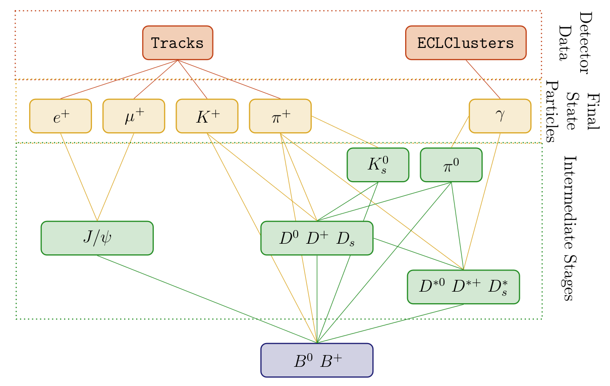
../../_images/hierarchy.png — Fig. 7.6 Hierarchical reconstruction applied by the FEI, which starting from tracks and EM clusters reconstructs initial state particles, intermediate particles in several stages and finally candidate $B$ tags.#

For instance, the FEI currently reconstructs 15 decay channels of the $D^{0}$ . Afterwards, the generated D0 candidates are used to reconstruct $D^{*0}$ in 2 decay channels. All information about the specific D0 decay channel of the candidate is encoded in its signal-probability, which is available to the $D^{*0}$ classifiers. In effect, the hierarchical approach reconstructs $2 * 15 = 30$ exclusive decay channels and provides a signal-probability for each candidate, which makes use of all available information. Finally, the $B$ candidates are reconstructed and the corresponding classifiers are trained. The final output of the FEI to the user contains four ParticleLists: B+:hadronic, B+:semileptonic, B0:hadronic and B0:semileptonic.

It is important to introduce intermediate cuts to reduce combinatorics in order to save computation time. The main goal of the cuts is to limit the combinatoric, while retaining the best $B$ meson candidates in each event. There are two types of cuts

PreCuts can be chosen for each channel individually and are done as early in the reconstruction as possible to save computing time.
PostCuts are applied after all information about the candidate from the vertex fitting and the MVC is available; The post-cut employs all available information about a candidate by cutting on the signal-probability calculated by the MVC. Since the interpretation of the signal probability is the same for all candidates independent of their decay channels the cut is channel-independent. It is important to choose this cut tight enough, otherwise one loses a lot of signal candidates in the consecutive reconstruction steps due to a bad signal-to-noise ratio

The FEI uses several cuts, which are applied for each particle in the following order:

PreCut::userCut is applied before all other cuts to introduce a-priori knowledge, e.g. final-state particle tracks (K shorts are handled via V0 objects) should originate from the IP '[dr < 2] and [abs(dz) < 4]', the invariant mass of D mesons should be inside a certain mass window '1.7 < M < 1.95', hadronic B meson candidates require a reasonable beam-constrained mass and delta E 'Mbc > 5.2 and abs(deltaE) < 0.5'. This cut is also used to enforce constraints on the number of additional tracks in the event for a specific signal-side 'nRemainingTracksInEvent == 1'.
PreCut::bestCandidateCut keeps for each decay channel only a certain number of best-candidates. The variable which is used to rank all the candidates in an event is usually the PID for final-state particles e.g. electronID, pionID, muonID`; the distance to the nominal invariant mass abs(dM) for intermediate particles; the product of the daughter SignalProbabilities for intermediate particles in semileptonic or KLong channels daughterProductOf(extraInfo(SignalProbability)). Between 10-20 candidates per channel (charge conjugated candidates are counted separately) are typically kept at this stage. This reduces the combinatoric in each event to the same level.
PreCut::vertexCut throws away candidates below a certain confidence level after the vertex fit. Default is throwing away only candidates with failed fits. Since the vertex fit is the most expensive part of the reconstruction it does not make sense to do a harder cut here, because the cuts on the network output afterwards will be more efficient without to much extra computing time
PostCut::value is a cut on the absolute value of the SignalProbability and should be chosen very loose, only candidates which are highly unlikely should be thrown away here
PostCut::bestCandidateCut keeps for each particle only a certain number of best-candidates. The candidates of all channels are ranked using their SignalProbability. Usually Between 10-20 candidates are kept per particle. This cut is extremely important because it limits the combinatoric in the next stage of reconstructions, and the algorithm can calculate the combinatoric at the next stage in advance.

Applying the FEI#

Just include the feistate.path created by the fei.get_path() function in your steering file.

The weightfiles are automatically loaded from the conditions database (see FEI and the conditions database). This might take some time.

After the FEI path the following lists are available

B+:generic (hadronic tag)
B+:semileptonic (semileptonic tag)
B0:generic (hadronic tag)
B+:semileptonic (semileptonic tag)

Each candidate has two extra infos which are interesting:

SignalProbability is the signal probability calculated using FastBDT
decayModeID is the tag $B$ decay channel

You can use a different decay channel configuration during the application. In particular you can omit decay channels (e.g. the semileptonic ones if you are only interested in the hadronic tag). However, it is not possible to add new channels without training them first (obviously).

You can find up to date examples in analysis/examples/FEI. If you encounter problems which require debugging in the FEI algorithm, the best starting point is to enable the monitoring, by choosing monitor=True in the FEIConfiguration. This will create a lot of root files containing histograms of interesting variables throughout the process (e.g. MC truth before and after all the cuts). You can also create a pdf using the root files produced by the monitoring and the “Summary.pickle” file produced by the original training by executing:

basf2 fei/latexReporting.py > summary.tex

FEI and the conditions database#

The FEI is frequently retrained and updated to give the best performance with the latest reconstruction, etc. You will need to use the relevant database in which the FEI training weights are located. FEI training weights are distributed by the basf2.conditions database under an analysis global tag. In order to find the latest, recommended FEI training, you can use the b2conditionsdb-recommend: Recommend a global tag to analyse a given file tool.

b2conditionsdb-recommend input_file.mdst.root

This tool will tell you all tags you should use. For the FEI we are only concerned with the analysis tag. Analysis tags are named analysis_tools_XXXX, and the latest and recommended one can be retrieved using the tool b2conditionsdb-recommend: Recommend a global tag to analyse a given file or the function modularAnalysis.getAnalysisGlobaltag. You will need to prepend this tag to your global tags list. This is done inside the FEI steering script.

import basf2
import fei

basf2.conditions.prepend_globaltag("analysis_tools_XXXX")
conf = fei.config.FeiConfiguration(prefix="foo", ...)

Note that when running on Belle converted data or MC you will need to use the B2BII and B2BII_MC database tags, respectively.

If you have trouble finding the correct analysis tag, please ask a question at B2Questions and/or send a mail to frank.meier@belle2.org,

Sphinx documentation#

Full Event Interpretation framework for Belle II

Detailed usage examples can be found in analysis/examples/FEI/

class fei.DecayChannel(name=None, label=None, decayString=None, daughters=None, mvaConfig=None, preCutConfig=None, decayModeID=None)#

Decay channel of a Particle.

daughters#: List of daughter particles of the decay channel e.g. [K+, pi-]

decayModeID#: DecayModeID of this channel. Unique ID for each channel of this particle.

decayString#: DecayDescriptor of the channel e.g. D0 -> K+ pi-

label#: Label used to identify the decay channel e.g. for weight files independent of decayModeID

mvaConfig#: MVAConfiguration object which is used for this channel.

name#

Name of the channel e.g. D0:generic_0

Type: str

preCutConfig#: PreCutConfiguration object which is used for this channel.

class fei.FeiConfiguration(prefix='FEI_TEST', cache=None, monitor=True, legacy=None, externTeacher='basf2_mva_teacher', training=False)#

Fei Global Configuration class

cache#: The stage which is passed as input, it is assumed that all previous stages do not have to be reconstructed again. Can be either a number or a filename containing a pickled number or None in this case the environment variable FEI_STAGE is used.

externTeacher#: Teacher command e.g. basf2_mva_teacher, b2mva-kekcc-cluster-teacher

legacy#: Pass the summary file of a legacy FEI training, and the algorithm will be able to apply this training.

monitor#: If true, monitor histograms are created

prefix#: The database prefix used for all weight files

training#: If you train the FEI set this to True, otherwise to False

class fei.FeiState(path, stage, plists)#

path#: Alias for field number 0

plists#: Alias for field number 2

stage#: Alias for field number 1

class fei.MVAConfiguration(method='FastBDT', config='--nTrees 400 --nCutLevels 10 --nLevels 3 --shrinkage 0.1 --randRatio 0.5', variables=None, target='isSignal', sPlotVariable=None)#

Multivariate analysis configuration class.

config#: Method specific configuration string passed to basf2_mva_teacher

method#: Method used by MVAInterface.

sPlotVariable#: Discriminating variable used by sPlot to do data-driven training.

target#: Target variable from the VariableManager.

variables#: List of variables from the VariableManager. {} is expanded to one variable per daughter particle.

class fei.Particle(identifier: str, mvaConfig: fei.config.MVAConfiguration, preCutConfig: fei.config.PreCutConfiguration = PreCutConfiguration(userCut='', vertexCut=- 2, noBackgroundSampling=False, bestCandidateVariable=None, bestCandidateCut=0, bestCandidateMode='lowest'), postCutConfig: fei.config.PostCutConfiguration = PostCutConfiguration(value=0.0, bestCandidateCut=0))[source]#

The Particle class is the only class the end-user gets into contact with. The user creates an instance of this class for every particle he wants to reconstruct with the FEI algorithm, and provides MVAConfiguration, PreCutConfiguration and PostCutConfiguration. These can be overwritten per channel.

addChannel(daughters: Sequence[str], mvaConfig: Optional[fei.config.MVAConfiguration] = None, preCutConfig: Optional[fei.config.PreCutConfiguration] = None)[source]#

Appends a new decay channel to the Particle object.

Parameters

daughters – is a list of pdg particle names e.g. [‘pi+’,’K-‘]
mvaConfig – multivariate analysis configuration
preCutConfig – pre cut configuration object

channels#: DecayChannel objects added by addChannel() method.

property daughters#: Property returning list of unique daughter particles of all channels

identifier#: pdg name of the particle with an optional additional user label separated by:

label#: Additional label like hasMissing or has2Daughters

mvaConfig#: multivariate analysis configuration (see MVAConfiguration)

name#: The name of the particle as correct pdg name e.g. K+, pi-, D*0.

postCutConfig#: post cut configuration (see PostCutConfiguration)

preCutConfig#: intermediate cut configuration (see PreCutConfiguration)

class fei.PostCutConfiguration(value=0.0, bestCandidateCut=0)#

PostCut configuration class. This cut is employed after the training of the mva classifier.

bestCandidateCut#: Number of best-candidates to keep, ranked by SignalProbability.

value#: Absolute value used to cut on the SignalProbability of each candidate.

class fei.PreCutConfiguration(userCut='', vertexCut=- 2, noBackgroundSampling=False, bestCandidateVariable=None, bestCandidateCut=0, bestCandidateMode='lowest')#

PreCut configuration class. These cuts is employed before training the mva classifier.

bestCandidateCut#: Number of best-candidates to keep after the best-candidate ranking.

bestCandidateMode#: Either lowest or highest.

bestCandidateVariable#: Variable from the VariableManager which is used to rank all candidates.

noBackgroundSampling#: For very pure channels, the background sampling factor is too high and the MVA can’t be trained. This disables background sampling.

userCut#: The user cut is passed directly to the ParticleCombiner. Particles which do not pass this cut are immediately discarded.

vertexCut#: The vertex cut is passed as confidence level to the VertexFitter.

fei.do_trainings(particles: Sequence[fei.config.Particle], configuration: fei.config.FeiConfiguration)[source]#

Performs the training of mva classifiers for all available training data, this function must be either called by the user after each stage of the FEI during training, or (more likely) is called by the distributed.py script after merging the outputs of all jobs,

Parameters

particles – list of config.Particle objects
config – config.FeiConfiguration object

Returns

list of tuple with weight file on disk and identifier in database for all trained classifiers

fei.get_default_channels(B_extra_cut=None, hadronic=True, semileptonic=True, KLong=False, baryonic=True, chargedB=True, neutralB=True, specific=False, removeSLD=False, strangeB=False)[source]#

returns list of Particle objects with all default channels for running FEI on Upsilon(4S). For a training with analysis-specific signal selection, adding a cut on nRemainingTracksInRestOfEvent is recommended.

Parameters

B_extra_cut – Additional user cut on recombination of tag-B-mesons
hadronic – whether to include hadronic B decays (default is True)
semileptonic – whether to include semileptonic B decays (default is True)
KLong – whether to include K_long decays into the training (default is False)
baryonic – whether to include baryons into the training (default is True)
chargedB – whether to recombine charged B mesons (default is True)
neutralB – whether to recombine neutral B mesons (default is True)
specific – if True, this adds isInRestOfEvent cut to all FSP
removeSLD – if True, removes semileptonic D modes from semileptonic B lists (default is False)
strangeB – if True, reconstruct B_s mesons in Upsilon5S decays (default is False)

fei.get_path(particles: Sequence[fei.config.Particle], configuration: fei.config.FeiConfiguration) → fei.core.FeiState[source]#

The most important function of the FEI. This creates the FEI path for training/fitting (both terms are equal), and application/inference (both terms are equal). The whole FEI is defined by the particles which are reconstructed (see default_channels.py) and the configuration (see config.py).

TRAINING For training this function is called multiple times, each time the FEI reconstructs one more stage in the hierarchical structure i.e. we start with FSP, pi0, KS_0, D, D*, and with B mesons. You have to set configuration.training to True for training mode. All weight files created during the training will be stored in your local database. If you want to use the FEI training everywhere without copying this database by hand, you have to upload your local database to the central database first (see documentation for the Belle2 Condition Database).

APPLICATION For application you call this function once, and it returns the whole path which will reconstruct B mesons with an associated signal probability. You have to set configuration.training to False for application mode.

MONITORING You can always turn on the monitoring (configuration.monitor = True), to write out ROOT Histograms of many quantities for each stage, using these histograms you can use the printReporting.py or latexReporting.py scripts to automatically create pdf files.

LEGACY This function can also use old FEI trainings (version 3), just pass the Summary.pickle file of the old training, and the weight files will be automatically converted to the new naming scheme.

Parameters

particles – list of config.Particle objects
config – config.FeiConfiguration object

fei.get_unittest_channels(specific=False)[source]#

Code structure#

In my opinion the best way to use and learn about the FEI is to read the code itself. I wrote an extensive documentation. Hence I describe here the code structure. If you don’t want to read code, you can just skip this part.

The FEI is completely written in Python and does only use general purpose basf2 modules. You can find the code under: analysis/scripts/fei/

config.py#

The classes defined here are used to uniquely define a FEI training.

The global configuration like database prefix, cache mode, monitoring, … (FeiConfiguration)
The reconstructed Particles (Particle)
The reconstructed Channels of each particle (DecayChannel)
The MVA configuration for each channel (MVAConfiguration)
The Cut definitions of each channel (PreCutConfiguration)
The Cut definitions of each particle (PostCutConfiguration)

These classes are used to define the default configuration of the FEI

default_channels.py#

Contains some example configurations of the FEI. Mostly you want to use get_default_channels(), which can return the configuration for common use-cases

Hadronic tagging (hadronic = True)
Semileptonic tagging (semileptonic = True)
B+/B- (chargedB = True)
B0/anti-B0 (neutralB = True)
running on Belle 1 MC/data (convertedFromBelle = True)
running a specific FEI which is optimized for a signal selection and uses ROEs (specific = True)

You can turn on and off individual parts of the reconstruction. I advise to train with the all parts, and then turn off the parts you don’t need in the application.

Another interesting configuration is given by get_fr_channels, which will return a configuration which is equivalent to the original Full Reconstruction algorithm used by Belle

In the training and application steering file you probably will use:

import fei
particles = fei.get_default_channels(hadronic=True, semileptonic=True, chargedB=True, neutralB=True)

core.py#

This file contains the implementation of the Full Event Interpretation Algorithm.

Some basic facts:

The algorithm will automatically reconstruct $B$ mesons and calculate a signal probability for each candidate.
It can be used for hadronic and semileptonic tagging.
The algorithm has to be trained on MC, and can afterwards be applied on data.
The training requires O(100) million MC events
The weightfiles are stored in the Belle II Condition database

Read this file if you want to understand the technical details of the FEI.

The FEI follows a hierarchical approach.

There are 7 stages:

(Stage -1: Write out information about the provided data sample)
Stage 0: Final State Particles (FSP)
Stage 1: $pi^{0}$, $J/\psi$ (and $Lambda^{0}$ if baryonic modes requested)
Stage 2: $K_{s}$ (and $Sigma^{+}$ if baryonic modes requested)
Stage 3: $D$ mesons (and $Lambda_{c}^{+}$ if baryonic modes requested)
Stage 4: $D^{*}$ mesons
Stage 5: $B$ mesons
Stage 6: Finish

Most stages consists of:

Create Particle Candidates
Apply Cuts
Do vertex Fitting
Apply a multivariate classification method
Apply more Cuts

The FEI will reconstruct these 7 stages during the training phase, since the stages depend on one another, you have to run basf2 multiple (7) times on the same data to train all the necessary multivariate classifiers.

Since running a 7-phase training by hand would be very difficult there is a tool which implements the training (including distributing the jobs on a cluster, merging the training files, running the training, …)

Training the FEI#

The FEI has to be trained on Monte Carlo data and is applied subsequently on real data after an analysis-specific signal-side selection. There are three different types of events one has to consider in the training and application of the FEI:

double-generic events - $e^{+}e^{-} \rightarrow \Upsilon(4S)\rightarrow B \bar{B}$ for charged and neutral B pairs, where both B mesons decay generically.
continuum events - $e^{+}e^{-} \rightarrow \Upsilon(4S)\rightarrow q \bar{q}$ where $q=u,d,s,c$.
and signal events - $e^{+}e^{-} \rightarrow \Upsilon(4S)\rightarrow B \bar{B}$, where one $B$ decays generically and the other decays in an analysis-specific signal-channel like $B^{+} \rightarrow \tau^{+} \nu_{\tau}$.

The final classifier output for the B tag mesons has to identify correctly reconstructed B tag mesons in the signal events of the analysis and reject background B tag mesons from double-generic, continuum and signal events efficiently. To accomplish a high efficiency for correctly reconstructed B tag in signal events a training on pure signal Monte Carlo after the signal-side selection would be appropriate, but in this scenario background components from double-generic and continuum events would not be considered in the training and therefore could not be rejected efficiently. On the other hand, a training on double-generic and continuum Monte Carlo after signal-side selection suffers from low statistics especially for correctly reconstructed B tag mesons, because the constraint that the reconstructed candidate has to use all remaining tracks is very strict. Moreover, it is not clear if D mesons from continuum background should be considered as signal in the corresponding trainings.

The background components are factorized into background from Υ(4S) decays and from continuum events. It is assumed that the continuum events can be suppressed efficiently with the ContinuumSuppression module, therefore no Monte Carlo data for continuum events is used in the training of the FEI. Further studies have to be performed to test this assumption.

The FR of Belle was trained on double-generic and continuum Monte Carlo without considering the signal-side selection. In consequence, the background distributions were fundamentally different in training and application. For example, most of the CPU time in the training was used for events with more than 12 tracks, yet these events never led to a valid $B$ tag meson in an analysis with only one track on the signal-side like $B^{+} \rightarrow \tau^{+} \nu_{\tau}$. Therefore the FEI employs two different training modes:

generic-mode; the training is done on double-generic Monte Carlo without signal-side selection, which corresponds to the FR of Belle. Hence, the training is independent of the signal-side and is only trained once for all analyses. The method is optimized to reconstruct tag-side of generic MC. If you don’t know your signal-side selection before the tag-side is reconstructed e.g. in an inclusive analysis like $B → X_c K$ or $B → X_{u/c} l \nu$, this is the mode you want.
specific-mode; the training is optimized for the signal-side selection and trained on double-generic and signal Monte Carlo, in order to get enough signal statistics despite the no-remaining-tracks constraint. In this mode the FEI is trained on the RestOfEvent after the signal-side selection, therefore the training depends on the signal-side and one has to train it for every analysis separately. The method is optimized to reconstruct the tag-side of signal MC. The usual tag-side efficiency is no longer a good measure for the quality, instead you have to look at the total Y4S efficiency including your signal-side efficiency. This mode can be used in searches for $B^{+} \rightarrow \tau^{+} \nu_{\tau}$ (Thomas Keck), $B^{+} \rightarrow l^{+} \nu_{l} \gamma$ (Moritz Gelb), $B^{0} \rightarrow \nu \bar{\nu}$ (Gianluca Inguglia), $B \rightarrow K^{*} \nu \bar{\nu}$, $B \rightarrow D^{*} \tau \nu_{\tau}$, … Another advantage is that global constraints on the beam-constrained mass and $\Delta E$ can be enforced at the beginning of the training.

In addition it is possible to train the multivariate classifiers for a decay channel on real data using sPlot, however I never tested it since we do not have real data (02/2016). We also trained the FEI successfully using Belle I MC. This is commonly known as “converted FEI”.

Basic Workflow (training)#

If you want to use the FEI in your analysis these are the steps you have to do (italic font refers only to specific-mode):

Get an account on KEKCC or access to another cluster where you can submit computing jobs. You will need 10-20 TB disk space during the training (we cache the reconstructed training data to save a lot of computing time)! Once the training is done you only need O(100MB) of data.
Locate the generic Monte Carlo from the current MC campaign, you will need ~100M Events (the more the better). Generate 50M-100M Monte Carlo events with one B decaying into your signal-channel, the other B decaying generically.
Create a new directory and two subdirectories named “collection” and “jobs”
Copy an example steering file from analysis/examples/FEI/ to your directory and modify it (especially choose a different prefix(!))
Use python3 analysis/scripts/fei/distributed.py to perform the training
Take a look at the summary.pdf which is created at the end of the training
Upload the weightfiles to the condition database: b2conditionsdb-request localdb/database.txt
Load the path in your analysis-steering file by choosing the option training=False in the FEIConfiguration
Use the ParticleLists created by the FEI B+:generic, B+:semileptonic, B0:generic, B0:semileptonic and the signal-probabilities stored in the extra Info (extraInfo(SignalProbability)) in your analysis.

In addition you may want to train the ContinuumSuppression separately and use it.

A typical training of the generic FEI will take about a week on the new KEKCC cluster using 100 cores and 100M events. The specific FEI can be trained much faster, but will require more statistics depending on your signal side selection

distributed.py#

This script can be used to train the FEI on a cluster like available at KEKCC. All you need is a basf2 steering file (see analysis/examples/FEI/ ) and some MC O(100) million

The script will automatically create some directories collection containing weightfiles, monitoring files and other stuff jobs containing temporary files during the training (can be deleted afterwards)

The distributed script automatically spawns jobs on the cluster (or local machine), and runs the steering file on the provided MC. Since a FEI training requires multiple runs over the same MC, it does so multiple times. The output of a run is passed as input to the next run (so your script has to use RootInput and RootOutput). In between it calls the do_trainings function of the FEI, to train the multivariate classifiers of the FEI at each stage. At the end it produces summary outputs using printReporting.py and latexReporting.py (this will only work of you use the monitoring mode). And a summary file for each mva training using basf2_mva_evaluate. If your training fails for some reason (e.g. a job fails on the cluster), the FEI will stop, you can fix the problem and resume the training using the -x option. This requires some expert knowledge, because you have to know how to fix the occurred problem and at which step you have to resume the training. After the training the weightfiles will be stored in the localdb in the collection directory. You have to upload these local database to the Belle II Condition Database if you want to use the FEI everywhere. Alternatively you can just copy the localdb to somewhere and use it directly, however, this is recommended only for testing as it is not reproducible.

You have to adjust the following parameters:

-n/--nJobs - the number of jobs which are submitted to the cluster. Every job has to process #input-files/nJobs data-files, so the number of jobs depend on the time-limit of each job on the cluster and the total number of files (assuming each file containing 1000 Events) you want to use for the training. On KEKCC nJobs=1000 for 100M Events (==100000 files) with a time limit of 3h on the short queue is sufficient.
-f/--steeringFile - the absolute path to the fei-training steering file.
-w/--workingDirectory - the absolute path to the working directory. This directory temporarily stores large training files, cut histograms, and other ntuples produced during the training of the FEI O(100GB).
-l/--largeDirectory - (optional) the absolute path to a directory with a lot of free space. The caching data O(10TB) is saved here, otherwise in the working directory.
-d/--data - The absolute paths to all your input files. You can use the bash glob expansion magic here (e.g. *)
-s/--site - The site you’re running on: At the moment kekcc, kitekp and local is supported.
-x/--skip-to - Skip to a specific step of the training. This is useful if you have to restart a training due to an earlier error (this is more an expert option).

Here’s a complete example:

python3 analysis/scripts/fei/distributed.py -s kekcc \
    -f analysis/examples/FEI/B_generic_train.py \
    -w /<local>/<path>/<to>/<project>/<directory>/ \
    -n 1000 -d /<local>/<path>/<to>/<input>/<mdst>/<files>/*.root

Known issues when training the FEI on the KEK system:

The automatic training can crash at several places. In most cases you hit a resource limit on your local machine or on your cluster

Disk space: Use df -h and du -sch to check this. Often this happens for directories that are not located at the HSM. E.g. the job directory due to large log files, or collection directory due to a large training file
Total number of processes: The FEI doesn’t use that much processes, still you can run into problems at KEKCC if other users use the machine in parallel.
CPU time on cluster: Make sure that each job has enough cpu time to finish before it is killed by the cluster-software. If the job on the first stage takes 15 minutes, intermediate stages can take up to ten times more!

Restarting a training#

If the training failed or you have to terminate a training temporarily you can usually restart it. The distributed script provides a option -x, which can restart the process at any point, and can even resubmit failed jobs.

I advise to take a look into the distributed.py script which is very well documented. Examples

You can find up to date examples in analysis/examples/FEI.

In general a FEI training steering file consists of

a decay channel configuration usually you can just use the default configuration in fei.get_default_channels. This configuration defines all the channels which should be reconstructed, the cuts, and the mva methods. You can write your own configuration, just take a look in analysis/scripts/fei/default_channels.py
a FeiConfiguration object, this defines the database prefix for the weightfiles and some other things which influence the training (e.g. if you want to run with the monitoring)
a feistate object, which contains the basf2 path for the current stage, you get this with the get_path function

The user is responsible for writing the input and output part of the steering file. Depending on the training mode (generic / specific) this part is different for each training (see below for examples). The FEI algorithm itself just assumes that the DataStore already contains a valid reconstructed event, and starts to reconstruct B mesons. During the training the steering file is executed multiple times. The first time it is called with the Monte Carlo files you provided, and the complete DataStore is written out at the end. The following calls must receive the previous output as input.

You can find up to date examples for training the specific or generic FEI, for the cases of Belle II of Belle converted data / MC in analysis/examples/FEI.

FEI Training on the Grid#

In this section, we will consider, how to run the FEI training workflow on the grid using gbasf2 and b2luigi.

Software and Environment Setup#

The following software packages need an installation: luigi, b2luigi, and gbasf2.

To profit from the latest developments of luigi and b2luigi, feel free to checkout the packages directly from github, as will be documented further below. You can also use particular releases of these packages to be installed with pip. Commands to install the two packages in your work directory from git are:

cd </path/to/your/work/directory>
mkdir -p sw; pushd sw
git clone https://github.com/spotify/luigi.git
git clone https://github.com/nils-braun/b2luigi.git
popd;

After this, you would need to setup the environment for python properly for these two packages with the following commands (they work only for bash):

export PATH="$(readlink -f sw)/luigi/bin:$PATH"
export PYTHONPATH="$(readlink -f sw)/luigi:$(readlink -f sw)/b2luigi:$PYTHONPATH"

Because of checking out the main branches of luigi and b2luigi, it might be that they do not work properly because of missing python packages. In that case, you can install them via the pip module:

python3 -m pip install colorama tenacity --user

The last step is to install gbasf2. For that purpose, please switch to a new terminal window with fresh environment on your machine, and follow the steps for gbasf2 installation.

In the following, an adaption for the gbasf2 package is discussed, which is required until the GitLab issue BIIDCD-1256 is resolved. It enables to upload non-basf2 data to remote SE’s on the grid.

Within the file BelleDIRAC/gbasf2/lib/ds/manager.py in function putDatasetMetadata(...), the lines

experiment_min, experiment_max = min(experiment_range), max(experiment_range)
run_min, run_max = min(run_range), max(run_range)

should be replaced with:

if len(experiment_range) > 0 and len(run_range) > 0:
    experiment_min, experiment_max = min(experiment_range), max(experiment_range)
    run_min, run_max = min(run_range), max(run_range)
else:
    experiment_min, experiment_max, run_min, run_max = -1, -1, -1, -1

After installing all prerequisites, you would need to get the example feiongridworkflow:

cd </path/to/your/work/directory>
git clone git@gitlab.desy.de:belle2/performance/fei/grid-workflow.git feiongridworkflow
cd feiongridworkflow

General Workflow Concept#

The b2luigi workflow of running FEI on the grid is constructed from 4 building blocks contained in fei_grid_workflow.py:

FEIAnalysisTask and FEIAnalysisSummaryTask: these tasks are performed to produce FEI training inputs based on mdst samples. They are used to run a basf2 steering file for FEI on the grid using gbasf2 as grid submission tool. In one instance of FEIAnalysisSummaryTask, several instances of FEIAnalysisTask are created, based on the provided dataset list. This allows to run this step on an unlimited number of input files.
MergeOutputsTask: After all outputs produced by FEIAnalysisSummaryTask are downloaded, they need to be merged into a single file to be able to run the MVA training on it.
FEITrainingTask: Performs the MVA training on merged outputs produced by MergeOutputsTask.
PrepareInputsTask: After a certain stage of MVA training is performed, all ingredients to produce FEI training inputs for the next stage require an upload to the grid storage elements. This is accomplished by this task, such that the FEIAnalysisSummaryTask can be run for the next stage based on these uploaded ingredients.

In the figure below, the concept of the workflow is visualized.

../../_images/FEI_Grid_Workflow.svg — Fig. 7.7 Visualization of the workflow concept of FEI training running on the grid.#

Starting with stage -1, at first the FEIAnalysisSummaryTask spawns several instances of FEIAnalysisTask, which are created for each individual line in the dataset list, assuming that one line is one dataset. In case of a file-based dataset processing, exactly one instance of FEIAnalysisTask is created for each dataset. In contrast to that, in case of an event-based processing, multiple instances of FEIAnalysisTask are created for each dataset, with the number of instances determined from the number of events to be processed at a certain stage. By the FEIAnalysisSummaryTask task, a cycle of four steps is started, containing FEIAnalysisSummaryTask at the beginning, followed by MergeOutputsTask, FEITrainingTask and PrepareInputsTask. As soon as FEIAnalysisSummaryTask is reached again, the stage number is increased by 1. This cycle is repeated until stage 5 is reached. Then, for stage 6, the workflow ends with FEITrainingTask.

Technical details#

In the following, more technical details will be discussed to be able to run the FEI on the grid.

settings.json#

The b2luigi configuration of the FEI grid workflow is handled by the file settings.json. Further below some explanations for the required settings:

gbasf2_install_directory: Absolute path to the directory where you have installed the gbasf2 tool. Please correct it to a meaningful path according to the installation you have performed previously.
gbasf2_input_dslist: Absolute path to the dataset list of all datasets you would like to process. It is assumed by the FEIAnalysisSummaryTask, that each line corresponds to a dataset sample, such that for each line in this dataset list one instance (file-based case) or multiple instances (event-based case) of FEIAnalysisTask are spawned. An example of a possible dataset list is given below:
/belle/MC/release-04-00-03/DB00000757/MC13a/prod00014078/s00/e0000/4S/r00000/mixed/mdst /belle/MC/release-04-00-03/DB00000757/MC13a/prod00014079/s00/e0000/4S/r00000/mixed/mdst /belle/MC/release-04-00-03/DB00000757/MC13a/prod00014088/s00/e0000/4S/r00000/charged/mdst /belle/MC/release-04-00-03/DB00000757/MC13a/prod00014089/s00/e0000/4S/r00000/charged/mdst
gbasf2_project_name_prefix: Prefix for the gbasf2 tasks which will be created by b2luigi in the FEI grid workflow. Please try to keep it short and it is recommended to you to attach a date to it. Within the workflow, an additional string _Part{index} will be added for each enumerated instance of FEIAnalysisTask, and b2luigi adds an additional hash number to the project name to keep it unique.
gbasf2_release: The release to be used on the grid. Please make a choice here depending on what is supported by the gbasf2 release you have checked out. You don’t have to worry about the case, that the developments in basf2 specific to running FEI training on the grid might not be contained in the official release. The FEI training steering file is adapted such, that it can run both with a development and an official release.
gbasf2_print_status_updates: Convenient option to monitor the progress of running gbasf2 tasks submitted by the FEI grid workflow, so it is good to set it to true. As an alternative, the progress can also be monitored with the Job Monitor application of Belle II DIRAC.
gbasf2_noscout: Option to disable scouting, which would slow down the progress, so it is set to true. Feel free to activate it for testing purposes.
gbasf2_basf2opt: To reduce the amount of print output of the gbasf2 jobs, this option should be set to "-l ERROR", which is then passed to the basf2 steering file. Having too many print outputs may cause problems on the grid worker nodes.
gbasf2_max_retries: An option that handles how often a job is allowed to be resubmitted, before its gbasf2 task is marked as failed in the b2luigi workflow. Since it is well possible that individual jobs fail due to connection issues or temporarily bad sites, it is good to set that option to a relatively high number, e.g. 5 or even 10. Of course, you are advised to have a look at log files of failed jobs in any case, e.g. by using Belle II DIRAC for that.
gbasf2_download_logs: To reduce the overall time of the FEI grid workflow, this option should be disabled by setting it to false. You can have a look at specific job logs by using Belle II DIRAC.
remote_tmp_directory: This option is used by the PrepareInputsTask to upload tarballs of input files required by FEIAnalysisTask running on the grid. The directory specified in this option serves as a main directory, where several subdirectories will be created by the uploads performed by PrepareInputsTask. To be able to access your temporary user folders on remote storage elements, the directory name should contain /belle/user/<your-grid-username>.
remote_initial_se: Initial storage element used by the PrepareInputsTask to upload the tarballs for the first time. After that first upload, the tarballs are replicated to storage elements corresponding to the ones, where the datasets specified in gbasf2_input_dslist are located. Possible initial storage element would be e.g. "KIT-TMP-SE".
local_cpus: Number of CPU’s used in parallel by the MergeOutputsTask on the local machine you are using. Please specify a sensible number, which does not lead to an overloaded machine.
working_dir, log_dir and result_dir: directories used by b2luigi for processing the specified workflow. In case of the FEI grid workflow, please choose a local storage element with enough space of at least several 100 GB.
executable: List of executables to be used for the b2luigi tasks, to be specified in this case to ["python3"].

B_generic_train.py#

In contrast to the original steering file from analysis/examples/FEI/B_generic_train.py, it is adapted to run both locally on your machine in the development setup of basf2, as well as to run on remote resources using an official basf2 release and a pickled path created from the steering file. To achieve this, two steps are performed:

The path creation is summarized in a corresponding function def create_fei_path(filelist=[], cache=0, monitor=False, verbose=False):, which returns a basf2 path. This function is then used within the b2luigi setup to create a corresponding fixed and pickled basf2 path.
The adaptions of histogram and n-tuple outputs needed for FEI training are reduced to a small set of files to avoid long lasting downloads of a large set of small files. In case these adaptions are not in an official release yet, which is supported by gbasf2, these need to be done by hand. This is accomplished within the for-loops for m in path.modules():.

FEIAnalysisSummaryTask and FEIAnalysisTask#

These modules are producing inputs for the FEI training. Since this is the most computationally intensive task, it is performed on the grid resources. The FEIAnalysisSummaryTask module is designed such, that it creates one instance (file-based case) or multiple instances (event-based case) of the FEIAnalysisTask module for each line entry in the dataset list given with the gbasf2_input_dslist setting. Each instance of FEIAnalysisTask is assigned with an individual dataset list containing the corresponding line entry and with a name modified with _Part{index}. In consequence, the module FEIAnalysisSummaryTask just summarizes the list of outputs produced by the individual tasks FEIAnalysisTask, saving the lists in the file list_of_output_directories.json.

Both modules have the following common settings:

cache: is used within the path creation of FEI steering file to configure, which inputs are already precomputed. In contrast to the procedure used by distributed.py, the only used values are -1 for stage -1 of FEI, and 0 for all other stages. This is done in that way to avoid large cache outputs RootOutput.root, which would require a lot of space on the grid. In consequence, to construct training data for a certain stage, all previous stages beginning from stage 0 need to be reconstructed from scratch using the corresponding trained BDTs that already exist.
monitor: is used within the path creation of FEI steering file to enable creation of ROOT files used for monitoring the training. This is essentially only required for the evaluation of trainings done during stage 6, and therefore is only enabled for that stage.
stage: is a task-specific setting to make a proper folder structure of the entire FEI training workflow. It is also used to set cache and monitor settings.
mode: is another task-specific setting to make a proper folder structure of the entire FEI training workflow. In case of FEIAnalysisSummaryTask, it is set to TrainingInput and extended with _Part{index} for the individual instances of FEIAnalysisTask.
gbasf2_project_name_prefix: taken from the settings.json for FEIAnalysisSummaryTask and is extended with _Part{index} for instances of FEIAnalysisTask. These prefixes are then used for the names of gbasf2 tasks created by the corresponding b2luigi batch process.
gbasf2_input_dslist: taken from settings.json for FEIAnalysisSummaryTask and is extended with _Part{index} for instances of FEIAnalysisTask. Corresponding individual dataset lists are created by FEIAnalysisSummaryTask.

The following outputs are produced by FEIAnalysisTask for different stages:

stage -1: mcParticlesCount.root summarizing the absolute number of produced particles on generator level
stages 0 to 5: training_input.root containing a flat n-tuple with variables required for the BDT training of a certain stage.
stage 6: Monitor*.root several output files with histograms, flat n-tuples or processing information to validate and evaluate the BDT trainings and the computational performance

To spawn several instances of FEIAnalysisTask at a certain stage, the following inputs are required to be already produced for stages greater -1:

Merged mcParticlesCount.root from stage -1.
All training files *.xml from previous stages.
Time stamp of inputs listed above, which were successfully uploaded to TMP-SE as a tarball by PrepareInputsTask of the previous stage.

During the sequential execution of all required instances of FEIAnalysisTask, symlinks are created for all input files (mcParticlesCount.root and *.xml, where applicable) to the current directory to correctly configure the basf2 path. The path is then pickled by b2luigi and send out to the grid with gbasf2 with an appropriate configuration of the grid path to the inputs tarball. The jobs are then monitored with corresponding gbasf2 tools and are resubmitted, if necessary. As soon as all jobs of an instance of FEIAnalysisTask are successfully completed, the job outputs required for further processing are downloaded.

In the current state of b2luigi, the workflow is interrupted, in case not all output files could be downloaded. In that case, you can resume the workflow (after checking the cause for the failed download) by simply restarting the workflow again and only the files for which the download failed will be downloaded.

The Problem of Too Long Runtimes#

One major drawback of the workflow presented here is that in particular the later stages of FEIAnalysisTask, beginning from stage 3 to stage 6, have large runtimes due to the fact, that most FEI stages have to be recomputed from scratch with the corresponding trainings applied, because cache output files RootOutput.root are not produced by the gbasf2 tasks since they occupy too much space.

This is a huge problem because of the fact, that individual jobs may fail for several reasons, causing potentially a large number of resubmission attempts. In consequence, a task submitted with gbasf2 to the grid may be delayed significantly by potentially only a few restarted jobs, which have to be run again for a long time.

A possible way out of this problem would be to split the processing per job by the number of events to be processed, and not by the number of files. This is not (yet) supported by gbasf2, but may be accomplished by passing -n and --skip-events options to basf2 via gbasf2_basf2opt of b2luigi. In that case, a gbasf2 task would need to be started for a single file only.

To realize this within the workflow constructed in fei_grid_workflow.py, the modules FEIAnalysisTask and FEIAnalysisSummaryTask are extended:

For FEIAnalysisSummaryTask, a stage dependent decision is taken, whether the jobs should be run on an entire file (file-based processing), or only on a subset of events from one single file (event-based processing). The configuration, whether to run a stage in a file-based or event-based manner is given in the dictionary processing_type in fei_grid_workflow.py:

processing_type = {
    -1: {"type": "file_based"},
{"type": "file_based"},
{"type": "file_based"},
{"type": "file_based"},
{"type": "event_based", "n_events": 50000},  # usually 1/4 of a file
{"type": "event_based", "n_events": 50000},  # usually 1/4 of a file
{"type": "event_based", "n_events": 20000},  # usually 1/10 of a file
{"type": "event_based", "n_events": 10000},  # usually 1/20 of a file
}

While stages -1 to 2 are fast enough to run them on an entire file, stages 3 to 6 should be run event-based by setting type to event_based. In that case, the number of events to be processed for a certain stage is configured by the key n_events in the processing_type dictionary. The configured numbers of events shown above are rough estimates to ensure, that the individual jobs run about 6 to 10 hours on a node. However, feel free to optimize these numbers and the choice of type of processing based on your own experience on the grid and your needs. If it is fine for you to run completely file-based, you can also set the type to file_based for all stages.

To determine, how many jobs should run for a single file to process all its events, a database is required for all files of the datasets to be used for training, which contains the information on the number of events per file. Since this information is required to create the workflow tree, and a b2luigi workflow is constructed in a deterministic manner, it is not possible to create the database at runtime of the different tasks spawned by the workflow. In consequence, this is implemented in the def requires(self): function of FEIAnalysisSummaryTask. This means, that the module FEIAnalysisSummaryTask with the largest stage number is creating this database to setup the instances of FEIAnalysisTask. All other modules FEIAnalysisSummaryTask with smaller stage numbers access the already created database to save time.

Technically, the gbasf2 tool gb2_ds_query_file is used to created this database called files_database.json, which is stored in the same directory as the dataset list configured with the gbasf2_input_dslist setting. Currently, this is taking some amount of time, in particular for a set of many large datasets, therefore this is only done once.

After the database files_database.json is created, the maximum number of events stored in the files is determined per dataset corresponding to a single line in the original dataset list. Based on these numbers, and the value of n_events in the processing_type dictionary for a considered stage, the number of instances of FEIAnalysisTask to be spawned is computed for each single dataset. Furthermore, the corresponding basf2 option values for -n and --skip-events, and a partial dataset list are constructed and then passed to the corresponding FEIAnalysisTask instance, which is extended with further properties process_events and skip_events to pass them to basf2.

The options -n and --skip-events of basf2 take care automatically of cases, when the number of remaining events to be processed from a file is smaller than configured by -n or the option --skip-events exceeds the maximum number of events in a file. In consequence, all files processed in an event-based manner are processed correctly. In summary, each instance of FEIAnalysisTask starts a gbasf2 task, which is configured to process all files from the assigned dataset, using the same fixed subset of events from the input files.

With this approach, the problem of too long runtimes per job is shifted to the requirement of having a large number of worker nodes in place to perform the computations and having a larger number of output files to be transferred in total. Since this is a grid workflow, this should be given in the ideal case. But be aware, that there are days, on which you get only a few free slots on the grid. Therefore, in case of central production of FEI training, a privileged access to the grid worker nodes would be very beneficial.

A potential and perhaps a bit more important problem of the event-based processing approach described above is a grid related issue of the current way of processing files placed on the grid. Currently, the files are not streamed, but copied completely to a worker node on the grid. In contrast to the file-based processing, where a single file is needed to be copied only once for an instance of FEIAnalysisTask, an event-based splitting may lead to multiple copy transfers of a single file, requested by multiple gbasf2 tasks at the same time. In consequence, if you specify too few events per job, a significant amount of jobs may fail at the beginning due to too many copy transfer requests for the same file. So please keep this in mind, when optimizing on a suitable number of events per job.

This problem might become less relevant, when input files are streamed and not copied, for example via XRootD transfers. Streaming via XRootD then usually takes care of transferring only the relevant information to the jobs, so only the events required by an instance of FEIAnalysisTask in case of event-based processing.

In the current state of b2luigi, the parallel instances of gbasf2 tasks (like FEIAnalysisTask in this workflow) are handled sequentially, and not in parallel. This means, that you should avoid creating too many tasks with the event-based splitting discussed above. So try to optimize in that case between the runtimes of single jobs and the total number of the tasks. However, in view of the fact, that this is done for stages 3 to 6, which anyhow run very long, this issue should not be a major problem.

MergeOutputsTask#

After all outputs from instances of FEIAnalysisTask are downloaded and listed by the FEIAnalysisSummaryTask in list_of_output_directories.json, the outputs from the various jobs need to be merged into a single file. This is accomplished by MergeOutputsTask using the information from list_of_output_directories.json and the (adapted) script analysis-fei-mergefiles from basf2.

This task depends on the FEIAnalysisSummaryTask running directly before it to be finished successfully, and has the following settings:

ncpus: number of CPUs of the local machine to be used for parallel merging, in case multiple outputs are produced by the gbasf2 tasks. The value is extracted from the settings.json (local_cpus).
monitor and stage: see description in FEIAnalysisSummaryTask and FEIAnalysisTask.

FEITrainingTask#

The BDT trainings of the various stages of FEI are performed by FEITrainingTask, after merged input for training was created by the corresponding MergeOutputsTask. This description fits the technical procedure exactly in case of stages 0 to 5.

For stage -1, the task is (ab)used to determine storage elements, where the input datasets given in gbasf2_input_dslist are located, and construct a list of sites (TMP-SE), where to put the tarballs created by instances of PrepareInputsTask.

In case of stage 6, all BDTs are already trained. Therefore, the merged Monitor*.root files are evaluated together with mcParticlesCount.root and *.xml files with the scripts analysis/scripts/fei/printReporting.py and analysis/scripts/fei/latexReporting.py within this task. As an additional validation step, the basf2_mva_evaluate.py script is used to process valid BDT *.xml training files using the merged training_input.root files from stages 0 to 5. For that purpose, these training_input.root files are merged into training_input_merged.root.

In consequence, the output produced by this module depends on the particular stage considered:

stage -1: dataset_sites.txt listing the TMP-SE sites to upload the tarball from PrepareInputsTask.
stages 0 to 5: *.xml BDT training files.
stage 6: summary.tex and summary.txt files, containing information on performance of FEI. The file summary.tex can then be compiled with pdflatex into a pdf document. In addition, training_input_merged.root is created for BDT evaluation, followed by *.zip outputs from this evaluation. For invalid BDT *.xml training files, zero-sized *.zip are created, as well as a zero-sized training_input_merged.root if all BDT trainings are invalid. This is done for the purpose of having the workflow finished successfully, since this is most probably not an intrinsic BDT training error, but an error due to low statistics.

Following inputs are required for FEITrainingTask depending on the current stage:

Merged mcParticlesCount.root from stage -1. This indicates also the dependence, that FEITrainingTask of stage -1 should start after MergeOutputsTask of stage -1 is successfully completed.
All training files *.xml from previous stages, in case BDT trainings were already performed.
Merged training_input.root from current stage, in case such a file was produced. This is true for stages 0 to 5.
Merged Monitor*.root from current stage, in case such a file was produced. This is true for stage 6.

For the required inputs listed above, symlinks are created to the current directory for stages 0 to 6. In case of merged training_input.root files from stages 0 to 5 to create training_input_merged.root, the paths to the original files are used directly to merge them.

To correctly configure the training for stages 0 to 5, the basf2 path needs to be created again to have the Summary.pickle file created, containing a local pickled version of the path. After that, the do_trainings(particles, configuration) function of the fei package is called to start BDT trainings needed for the current stage.

For stage 6, the scripts analysis/scripts/fei/printReporting.py and analysis/scripts/fei/latexReporting.py are executed on top of the inputs provided via symlinks, and the script basf2_mva_evaluate.py on training_input_merged.root.

Also for this module, the usual parameters are used to define the folder structure of outputs:

monitor and stage: see description in FEIAnalysisSummaryTask and FEIAnalysisTask.

PrepareInputsTask#

After FEITrainingTask is finished successfully, the last step before increasing the stage and starting again from FEIAnalysisSummaryTask is an upload of all inputs required for instances of FEIAnalysisTask to the storage elements where the datasets are located.

To be able to upload necessary files to SE, the following inputs are required:

dataset_sites.txt from FEITrainingTask of stage -1 which contains all sites required for tarball replicas.
Merged mcParticlesCount.root from stage -1. This indicates also the dependence, that FEITrainingTask of stage -1 should start after MergeOutputsTask of stage -1 is successfully completed.
All training files *.xml from previous stages and current stage, in case BDT trainings were already performed.

The files mcParticlesCount.root and *.xml are then put into a tarball, copied over by gbasf2 tools to the initial TMP-SE storage element configured in settings.json., and then the tarball is replicated to the storage elements from dataset_sites.txt. In case of a successful upload and replication, the timestamp used in the remote path of the tarball is written to successful_input_upload.txt, which is checked by the FEIAnalysisSummaryTask directly following this PrepareInputsTask.

The following parameters are used in this module:

remote_tmp_directory: TMP-SE directory, where to put the tarballs. Extracted from settings.json.
remote_initial_se: TMP-SE server, where the tarballs should be put at first to be used for replication. Extracted from settings.json.
monitor and stage: see description in FEIAnalysisSummaryTask and FEIAnalysisTask.

Further Comments on fei_grid_workflow.py#

To run the workflow chain prepared in fei_grid_workflow.py, you would need to start it from the last task in this workflow that you would like to consider. From that point on, all other tasks will be constructed from the requirements, down to the FEIAnalysisSummaryTask of stage -1. This can be done with the wrapper task called ProduceStatisticsTask.

To run the full workflow, the wrapper contains the following piece of code:

yield FEITrainingTask(
    mode="Training",
    stage=6,
)

For testing purposes, feel free to change it to a different step in the workflow. Examples are given as comments within the ProduceStatisticsTask module. Please also note, that the names of the mode and stage settings should be chosen as expected by the modules to setup the considered workflow correctly.

Tips and Tricks#

In this concluding section of running FEI training on the grid, a few tips and tricks are given, such that you get a better feeling what to expect from the workflow and which pitfalls you may encounter, especially when running on the grid.

In general, you should always test the setup locally before submitting it to the grid. Therefore, please adapt your steering file equivalent to B_generic_train.py in such a way, that you would be able to run it both locally (potentially with a development version of basf2) and on the grid (using an official basf2 release).
To test the workflow on the grid in a fast way, you can construct the dataset list provided to the gbasf2_input_dslist setting using individual file paths as content instead of dataset paths, and setting the maximum number of events to a small value, e.g. 10. There are several possibilities to do that. You can either set it directly for the FEIAnalysisTask using the max_event task parameter (see b2luigi documentation), or extend the setting gbasf2_basf2opt from "-l ERROR" to "-l ERROR -n 10". The training itself will then have no meaning, since too few events for training, but you would be able to test the technical setup with that approach.
To run instances of FEIAnalysisTask efficiently on the grid, you should prepare yourself well for that.
- You should make sure, that the datasets you would like to process are available on as many sites as possible. In that way you would also increase the number of potential computing nodes on the grid that you can use.
- In case you would like to perform a central FEI training, which will then be provided centrally and used by several analysis groups, it would be good, that your jobs will get an increased priority on the grid to allow you to get the resources you need faster.
- If you do not trust some computing sites, or you trust only a few, you can make use of gbasf2_additional_params setting of b2luigi to ban some sites ("--banned_site <SITE-1,SITE-2>") or specify sites you would like to run on ("--site <SITE-1,SITE-2>"). The value of the parameter gbasf2_additional_params will then be passed to gbasf2.
Although the workflow is (more or less) automatic, you are strongly advised to have a look at its progress regularly and check, whether everything is done correctly and do not run it as a black box.
Please expect, that problems may arise during the process, because of (possible temporarily) bad state of sites, failing downloads due to connection problems etc. Individual jobs may need to be resubmitted several times until they are finished successfully.
In case you encounter problems specific to gbasf2, do not hesitate to ask experts on the comp-users-forum mailing list.

Possible Improvements#

Some ideas of improvements of the workflow constructed to run the FEI training on the grid will be given below.

Potential Improvements Following gbasf2 Development#

In the current state of the workflow and b2luigi, some print outputs from gbasf2 have to be parsed to obtain desired information. Depending on the future improvements of gbasf2, such parsing may be changed to a more convenient way, for example parsing a json file output created by gbasf2 tools on request.

According to the discussions with gbasf2 developers, developments are ongoing to allow the gbasf2 tasks to save the sandbox not on a central server, but distributed on several storage sites. This would allow to use the option --input_sandboxfiles of gbasf2 to take care of uploading the inputs collected currently by the PrepareInputsTask. The reason for doing it currently with PrepareInputsTask by hand, is that the sandbox is not allowed to exceed the size of 10 MB. As soon as the distribution of the sandbox among multiple storage elements is introduced to gbasf2, the option --input_sandboxfiles can then be used directly and this would make the module PrepareInputsTask obsolete.

Another possible improvement of gbasf2 which is currently considered by the developers is the possibility to start merging jobs on the grid. This would allow for performing MergeOutputsTask on the grid with the potential to speed up this part of the workflow, avoiding the time spent for downloads and merging on the local machine.

In general, it is good to have a look at the process of gbasf2 developments and extend the workflow and/or b2luigi to make use of the new features and improvements of future gbasf2 releases. One example would be the possibility to resubmit jobs with changed settings, e.g. sites to reject, and/or the estimated runtime of the job.

Troubleshooting#

Crash in the Neurobayes Library#

The mva package NeuroBayes is used in the KShort Finder of the belle software. However, NeuroBayes is no longer officially supported by the company who developed it and also not by the Belle II collaboration. Nevertheless, you still need it to run b2bii.

There is a working neurobayes installation at KEKCC which you can use. This does mean that you can only use b2bii (and in consequence the FEI on converted MC) if you work on KEKCC.

If you are on KEKCC and get a crash you probably forgot to set the correct LD_LIBRARY_PATH

export LD_LIBRARY_PATH=/sw/belle/local/neurobayes/lib/:$LD_LIBRARY_PATH

You have to set this AFTER you set up basf2, otherwise basf2 will override the LD_LIBRARY_PATH again.

Note that the NeuroBayes libraries which are shipped with the basf2 externals are only dummy libraries which are used during the linking of b2bii. They do not contain any NeuroBayes code, only functions with the correct signatures which will crash if they are called. Therefore it is important that the correct NeuroBayes libraries are found by the runtime-linker BEFORE the libraries shipped with basf2. This means you have to add the neurobayes path before the library path of the externals.

Running FEI on converted Belle MC outside of KEK#

There are two problems with this:

You don’t have access to the old Belle condition database outside of KEK
You don’t have access to the NeuroBayes installation outside of KEK

To access the old Belle database anyway you have to forward to server to you local machine and set the environment variables correctly

ssh -L 5432:can01kc.cc.kek.jp:5432 tkeck@cw02.cc.kek.jp

export BELLE2_FILECATALOG=NONE

export USE_GRAND_REPROCESS_DATA=1

export PGUSER=g0db

export BELLE_POSTGRES_SERVER=localhost

Depending on how you use b2bii, the BELLE_POSTGRES_SERVER will be overridden by b2bii. Hence you have to enforce that localhost is used anyway. You can ensure this by adding:

import os

os.environ['BELLE_POSTGRES_SERVER'] = 'localhost'

directly before you call process().

The second problem is more difficult. You require a neurobayes installation. On KEKCC the installation is here /sw/belle/local/neurobayes/, and you might be tempted to copy the files from here and to run it on your local machine. However you require a license to run neurobayes on your machine. Since the latest neurobayes release 4.3.1 this license requirement is no longer technically enforced.

Neurobayes versions for Ubuntu (instead of SL6) are available as well.

Anyway don’t forget to add neurobayes to your LD_LIBRARY_PATH after(!) you set up basf2

export LD_LIBRARY_PATH=/sw/belle/local/neurobayes/lib/:$LD_LIBRARY_PATH

Btw, the Neurobayes libraries which are shipped with the basf2 externals are only dummy libraries which will just crash if you try to use them. They are only used so everybody can compile b2bii (because you require the libraries to link the b2bii modules).

Speeding up the FEI#

The FEI is optimized for maximum speed, but the default configuration is not suitable for all applications. This means, one can save a lot of computing time. Here is a short list of things you can do to speed up the application of the FEI.

Use Fast Fit instead of KFit will gain a factor 2.
Deactivate the reconstruction unused B lists (by default hadronic, semileptonic, charged and neutral are all created) (see analysis/script/fei/default_channels.py). The get_default_channels function has parameters for this.
If you use the semileptonic tag but don’t want to use semileptonic D decays, you can deactivate them. But you have to comment out the corresponding channels in the get_default_channels function, or create your own custom channel configuration.
Add extra cuts before the combination of the B mesons, e.g. the cut on Mbc is by default for hadronic B mesons only >5.2. There is a parameter called B_extra_cut in the get_default_channels function.
Add a skim cut on the number of tracks. Just add an applyEventCuts to your path before running the FEI. In fact, the maximum number of tracks for a correct B candidate is 7 (not in theory, but in practice). Hence, If you know you only want one track on the signal side. You can discard all events with more than 8 tracks from the beginning, without losing any correctly reconstructed signal events. This is of course not possible for an inclusive signal-side.

With FEIv4 you don’t need to re-train anything if you apply the above mentioned changes. Deactivating channels and tightening cuts is fine. For instance, I made a large study on the influence of the track-cut described above, and it doesn’t matter at all if you use choose a different cut than the one used during the training.

Resources, Publications etc.#

The Full Event Interpretation – An exclusive tagging algorithm for the Belle II experiment
Belle II “Full Event Interpretation” publication
Improvement of the Full Reconstruction of B Mesons at the Belle Experiment
Fabian’s diploma thesis. This thesis contains a description of the importance of various channels in Appendix B
Search for B –> h nu nu decays at Belle
Oksana’s doctoral thesis. This thesis is one of the “poster analyses”, we have done in Karlsruhe, which shaped our understanding of Full Reconstruction analysis.
The Full Event Interpretation for Belle II
Thomas’s master thesis. Describes the proof-of-concept implementation of the FEI in Belle II, this twiki page is in large parts copied from here.
Machine learning algorithms for the Belle II experiment and their validation on Belle data
Thomas’s PhD thesis.

basf2 development documentation

Full event interpretation

Contents

7.8.5. Full event interpretation#

Algorithm overview#

Physics#

Key Performance Indicators#

Hadronic, Semileptonic and Inclusive Tagging#

Hierarchical Approach#

Applying the FEI#

FEI and the conditions database#

Sphinx documentation#

Code structure#

config.py#

default_channels.py#

core.py#

Training the FEI#

Basic Workflow (training)#

distributed.py#

Restarting a training#

FEI Training on the Grid#

Software and Environment Setup#

General Workflow Concept#

Technical details#

settings.json#

B_generic_train.py#

FEIAnalysisSummaryTask and FEIAnalysisTask#

The Problem of Too Long Runtimes#

MergeOutputsTask#

FEITrainingTask#

PrepareInputsTask#

Further Comments on fei_grid_workflow.py#

Tips and Tricks#

Possible Improvements#

Potential Improvements Following gbasf2 Development#

Troubleshooting#

Crash in the Neurobayes Library#

Running FEI on converted Belle MC outside of KEK#

Speeding up the FEI#

Resources, Publications etc.#