
3.4.11. ONNX MVA tutorial#
Note
This tutorial closely follows the Continuum suppression using Boosted Decision Trees tutorial. If you are new to either Continnum suppression or Machine Learning in general read that one first.
Intended audience
This tutorial is directed towards analyzers who wish to use custom machine learning methods (e.g. with libraries like scikit-learn, tensorflow, torch, xgboost, lightgbm, …) and still want to apply inference with the resulting trained models within basf2. The tutorial uses scikit-learn, but the general approach should be applicable to other libraries as well.
The recommended way to run inference with custom machine learning methods in basf2 is via ONNX. In this tutorial we will use the ONNX method within the MVA package. That means we don’t write any basf2 modules, but will use the existing functionality from the MVAExpert module and only write steering files.
Creating an ntuple with training data#
We will start by creating an ntuple for training our ML model with the following steering file - it’s identical to the one in Continuum suppression using Boosted Decision Trees, but we will process all events since we intend to split between train and test dataset in the custom ML part outside basf2.
#!/usr/bin/env python3
import basf2 as b2
import modularAnalysis as ma
import stdPi0s

# Perform analysis.
main = b2.create_path()

ma.inputMdstList(
    filelist=[
        b2.find_file(
            "starterkit/2021/B02ks0pi0_sample.root", data_type="examples"
        ),
        b2.find_file("starterkit/2021/uubar_sample.root", data_type="examples"),
    ],
    path=main,
)

stdPi0s.stdPi0s(path=main, listtype="eff60_May2020")
ma.fillParticleList(
    decayString="pi+:good", cut="chiProb > 0.001 and pionID > 0.5", path=main
)

ma.reconstructDecay(
    decayString="K_S0 -> pi+:good pi-:good", cut="0.480<=M<=0.516", path=main
)

ma.reconstructDecay(
    decayString="B0  -> K_S0 pi0:eff60_May2020",
    cut="5.1 < Mbc < 5.3 and abs(deltaE) < 2",
    path=main,
)

ma.buildRestOfEvent(target_list_name="B0", path=main)
cleanMask = (
    "cleanMask",
    "nCDCHits > 0 and useCMSFrame(p)<=3.2",
    "p >= 0.05 and useCMSFrame(p)<=3.2",
)
ma.appendROEMasks(list_name="B0", mask_tuples=[cleanMask], path=main)

ma.buildContinuumSuppression(list_name="B0", roe_mask="cleanMask", path=main)

simpleCSVariables = [
    "R2",
    "thrustBm",
    "thrustOm",
    "cosTBTO",
    "cosTBz",
    "KSFWVariables(pt_sum)",
    "KSFWVariables(mm2)",
    "KSFWVariables(hso00)",
    "KSFWVariables(hso01)",
    "KSFWVariables(hso02)",
    "KSFWVariables(hso03)",
    "KSFWVariables(hso04)",
    "KSFWVariables(hso10)",
    "KSFWVariables(hso12)",
    "KSFWVariables(hso14)",
    "KSFWVariables(hso20)",
    "KSFWVariables(hso22)",
    "KSFWVariables(hso24)",
    "KSFWVariables(hoo0)",
    "KSFWVariables(hoo1)",
    "KSFWVariables(hoo2)",
    "KSFWVariables(hoo3)",
    "KSFWVariables(hoo4)",
    "CleoConeCS(1)",
    "CleoConeCS(2)",
    "CleoConeCS(3)",
    "CleoConeCS(4)",
    "CleoConeCS(5)",
    "CleoConeCS(6)",
    "CleoConeCS(7)",
    "CleoConeCS(8)",
    "CleoConeCS(9)",
]

ma.variablesToNtuple(
    decayString="B0",
    variables=simpleCSVariables + ["Mbc", "isContinuumEvent"],
    filename="ContinuumSuppression.root",
    treename="ntuple",
    path=main,
)

b2.process(main)
Train a BDT classifier with scikit-learn#
It works without any basf2 dependencies, so for simplicity we run it in an isolated environment, e.g. using uv:
uv venv
source .venv/bin/activate
uv pip install scikit-learn matplotlib pandas uproot awkward-pandas \
    skl2onnx onnxmltools onnx onnxruntime netron jupyter

jupyter lab
So for this tutorial we need to keep one terminal with a basf2 environment open for executing steering files and code that needs basf2 and have jupyter running in the isolated environment in a second terminal.
First, we load our ntuple into a pandas DataFrame:
import uproot

with uproot.open({"ContinuumSuppression.root": "ntuple"}) as tree:
    df = tree.arrays(library="pd")
    # undo the replacement for the brackets in variable names
    df.columns = [col.replace("__bo", "(").replace("__bc", ")") for col in df.columns]
Now, we prepare input and output arrays and split randomly 50:50 into train and test datasets:
variables = [
    "R2",
    "thrustBm",
    "thrustOm",
    "cosTBTO",
    "cosTBz",
    "KSFWVariables(pt_sum)",
    "KSFWVariables(mm2)",
    "KSFWVariables(hso00)",
    "KSFWVariables(hso02)",
    "KSFWVariables(hso04)",
    "KSFWVariables(hso10)",
    "KSFWVariables(hso12)",
    "KSFWVariables(hso14)",
    "KSFWVariables(hso20)",
    "KSFWVariables(hso22)",
    "KSFWVariables(hso24)",
    "KSFWVariables(hoo0)",
    "KSFWVariables(hoo1)",
    "KSFWVariables(hoo2)",
    "KSFWVariables(hoo3)",
    "KSFWVariables(hoo4)",
    "CleoConeCS(1)",
    "CleoConeCS(2)",
    "CleoConeCS(3)",
    "CleoConeCS(4)",
    "CleoConeCS(5)",
    "CleoConeCS(6)",
    "CleoConeCS(7)",
    "CleoConeCS(8)",
    "CleoConeCS(9)",
]

X = df[variables].to_numpy()
y = df["isContinuumEvent"].to_numpy()

from sklearn.model_selection import train_test_split

X_train, X_test, y_train, y_test = train_test_split(X, y, test_size=len(X) // 2, random_state=42)
We will use the HistGradientBoostingClassifier in default settings from scikit-learn for this exercise
from sklearn.ensemble import HistGradientBoostingClassifier

bdt = HistGradientBoostingClassifier()
bdt.fit(X_train, y_train)
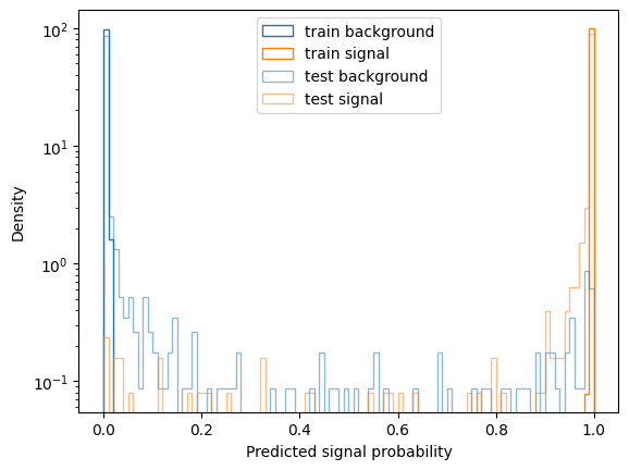
For a quick evaluation we plot the distribution of predicted probabilities for train and test set:
import matplotlib.pyplot as plt

p_train = bdt.predict_proba(X_train)[:, 1]
p_test = bdt.predict_proba(X_test)[:, 1]

def plot(p, y, **kwargs):
    label = kwargs.pop("label", "")
    kwargs = dict(kwargs, bins=100, range=(0, 1), histtype="step", density=True)
    plt.hist(p[y==0], color="C0", label=f"{label} background", **kwargs)
    plt.hist(p[y==1], color="C1", label=f"{label} signal", **kwargs)
    plt.yscale("log")

plot(p_train, y_train, label="train")
plot(p_test, y_test, alpha=0.5, label="test")
plt.xlabel("Predicted signal probability")
plt.ylabel("Density")
plt.legend()
And we also look at the ROC curves:
from sklearn.metrics import roc_curve, roc_auc_score

plt.plot(*roc_curve(y_train, p_train)[:2], label="train")
plt.plot(*roc_curve(y_test, p_test)[:2], label="test")
plt.xlabel("False positive rate")
plt.ylabel("True positive rate")
plt.legend()
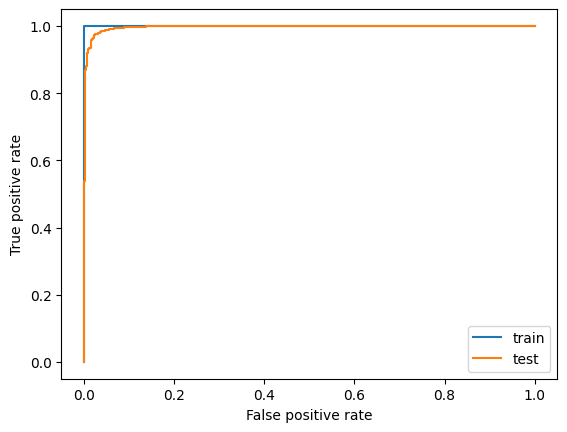
roc_auc_score(y_test, p_test)
0.9961197133415023
All in all we see the classifier is pretty overtrained on this rather small dataset (roughly 2000 events), but still the Area Under Curve (AUC) score is quite high for the test data set still. Optimizing the Hyperparameters of the model probably does not make too much sense at this point - we would first try to gather a larger data sample.
Convert the scikit-learn model to ONNX#
Now, to be able to run inference for this model within basf2 we have to convert it to ONNX. We will use skl2onnx, which provides conversion for most models within scikit-learn
The option {"zipmap": False} is necessary to get an ONNX model that outputs a single tensor. Consult the corresponding section in the skl2onnx documentation for more information.
Now, we can visuzualize the model graph using netron. We can either load our model in the web application or in a jupyter notebook we can run a widget via
import netron

netron.widget(netron.start("bdt.onnx", browse=False))

The graph has 2 output tensors, named “probabities” and “label” - we will only use the “probabilities”. That tensor has shape (?, 2) for which the MVA ONNX method will by default pick the second output (index 1) as the signal class when run in non-multiclass mode (which will be used in the MVAExpert module when we have a binary classifier). The index is also configurable via the signal_class option in the weightfile.
Before we run this through basf2, let’s quickly cross check if the outputs from the sklearn model and the ONNX model match reasonably close:
import onnxruntime as ort
import numpy as np

session = ort.InferenceSession("bdt.onnx")
p_test_onnx = session.run(["probabilities"], {"input": X_test.astype(np.float32)})[0][:, 1]

np.allclose(p_test_onnx.ravel(), p_test, atol=1e-4)
True
Matches with absolute differences between 1e-3 and 1e-5 are typical. In general one should validate if this leads to the same performance - we will do that shortly after having run the model in basf2.
Save model to MVA Weightfile and run in basf2#
We can now store the ONNX model in a MVA Weightfile:
# this code has to run in a basf2 environment
from basf2_mva_util import create_onnx_mva_weightfile

# variables = [...] # copy this from above

weightfile = create_onnx_mva_weightfile(
    "bdt.onnx",
    outputName="probabilities",
    variables=variables,
    target_variable="isContinuumEvent",
)
weightfile.save("MVA_ONNX_BDT.root")
Now, we can run a steering file that applies our model and dumps a new ntuple with the model outputs included:
#!/usr/bin/env python3

import basf2 as b2
import modularAnalysis as ma
import stdPi0s
from variables import variables as vm

main = b2.create_path()

ma.inputMdstList(
    filelist=[
        b2.find_file(
            "starterkit/2021/B02ks0pi0_sample.root", data_type="examples"
        ),
        b2.find_file("starterkit/2021/uubar_sample.root", data_type="examples"),
    ],
    path=main,
)

stdPi0s.stdPi0s(path=main, listtype="eff60_May2020")
ma.fillParticleList(
    decayString="pi+:good", cut="chiProb > 0.001 and pionID > 0.5", path=main
)
ma.reconstructDecay(
    decayString="K_S0 -> pi+:good pi-:good", cut="0.480<=M<=0.516", path=main
)
ma.reconstructDecay(
    decayString="B0  -> K_S0 pi0:eff60_May2020",
    cut="5.1 < Mbc < 5.3 and abs(deltaE) < 2",
    path=main,
)
ma.buildRestOfEvent(target_list_name="B0", path=main)
cleanMask = (
    "cleanMask",
    "nCDCHits > 0 and useCMSFrame(p)<=3.2",
    "p >= 0.05 and useCMSFrame(p)<=3.2",
)
ma.appendROEMasks(list_name="B0", mask_tuples=[cleanMask], path=main)
ma.buildContinuumSuppression(list_name="B0", roe_mask="cleanMask", path=main)

main.add_module(
    "MVAExpert",
    listNames=["B0"],
    extraInfoName="ContinuumProbability",
    identifier="MVA_ONNX_BDT.root",  # name of the weightfile used
)

vm.addAlias("ContProb", "extraInfo(ContinuumProbability)")
ma.variablesToNtuple(
    decayString="B0",
    variables=["ContProb", "isContinuumEvent"],
    filename="ContinuumSuppression_applied.root",
    treename="ntuple",
    path=main,
)

b2.process(main)
Again, we run over all events and for the purpose of this demonstration we only write out the inference results.
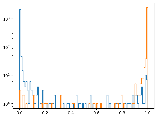
We can now cross check the result in our notebook:
with uproot.open({"ContinuumSuppression_applied.root": "ntuple"}) as tree:
    df = tree.arrays(library="pd")

np.allclose(df["ContProb"].to_numpy(), bdt.predict_proba(X)[:, 1], atol=1e-4)
True
And have a look at the output distributions - note this is now train and test sample merged:
p_mva = df["ContProb"].to_numpy()

kwargs = dict(bins=100, range=(0, 1), histtype="step")
plt.hist(p_mva[y==0], **kwargs)
plt.hist(p_mva[y==1], **kwargs)
plt.yscale("log")
Run the basf2 mva evaluation#
We can also run the basf2_mva_evaluate.py script. To do so we first create ntuples from our notebook to reflect the same train/test splitting we have actually used for our training:
import pandas as pd
root_variables = [var.replace("(", "__bo").replace(")", "__bc") for var in variables]

def write_rootfile(X, y, filename):
    df = pd.DataFrame(X, columns=root_variables)
    df["isContinuumEvent"] = y
    with uproot.recreate(filename) as f:
        f["ntuple"] = df

write_rootfile(X_train, y_train, "train.root")
write_rootfile(X_test, y_test, "test.root")
Now we can run the evaluation and enjoy the plots - the probability output distributions and ROC curves should look familiar 🙂
basf2_mva_evaluate.py -id MVA_ONNX_BDT.root -train train.root -data test.root -o evaluate.zip